AWS Announces General Availability of Amazon Security Lake

Amazon Web Services (AWS) has recently announced the general availability of Amazon Security Lake, a service that automatically centralises an organisation’s security data from across their AWS environments, leading SaaS providers, on-premises environments, and cloud sources into a purpose-built data lake, so customers can act on security data faster and simplify security data management across hybrid and multi-cloud environments.

Amazon Security Lake is generally available today in US East (Ohio), US East (N. Virginia), US West (Oregon), Asia Pacific (Singapore), Asia Pacific (Sydney), Asia Pacific (Tokyo), Europe (Frankfurt), Europe (Ireland), Europe (London), and South America (São Paulo) with availability in additional AWS Regions coming soon.

Amazon Security Lake converts and conforms incoming security data to the Open Cybersecurity Schema Framework (OCSF) open standard, making it easier for security teams to automatically collect, combine, and analyse security data from more than 80 sources, including AWS, security partners, and analytics providers.

Amazon Security Lake is part of a broad set of AWS Cloud security services that build on AWS’s secure infrastructure to help make it the most flexible and secure cloud trusted by millions of customers, including some of the most security-sensitive organisations, and is supported by a broad community of security partners to help customers elevate their security in the cloud.

“Security has been our top priority since the very beginning, when we were designing to meet the needs of the most security-sensitive organisations. We also know that customers need trusted partners to extend the benefits of the cloud and make sure their organisations are secure end-to-end.

“With more than 80 sources providing data to Amazon Security Lake, security teams can achieve greater visibility into potential security threats and how to respond to them, further protecting the workloads, applications, and data that are critical to driving business forward,” Jon Ramsey, vice president for Security Services at AWS, said.

The post AWS Announces General Availability of Amazon Security Lake appeared first on Analytics India Magazine.

Advanced Feature Selection Techniques for Machine Learning Models

Advanced Feature Selection Techniques for Machine Learning Models
Image by Author

Machine learning is undeniably the shining star of the new era. It forms the backbone of various major technologies that have become integral to our daily lives, such as facial recognition (supported by Convolutional Neural Networks or CNN), speech recognition (leveraging CNN and Recurrent Neural Networks or RNN), and the increasingly popular chatbots like ChatGPT (powered by Reinforcement Learning from Human Feedback, RLHF).

Numerous methods are available today to enhance the performance of a machine learning model. These methods can give your project a competitive edge by delivering superior performance.

In this discussion, we'll delve into the realm of feature selection techniques. But before we proceed, let's clarify: what exactly is feature selection?

What Is the Feature Selection?

Feature selection is the process of choosing the best features for your model. This process might differ from one technique to another, but the main goal is to find out which features have more impact on your model.

Why Should We Do Feature Selection?

Because sometimes, having too many features might harm your machine learning model. How?

There might be too many different reasons. For example, these features might be related to each other, which can cause multicollinearity, ruining your model’s performance.

Another potential issue is related to computational power. The presence of too many features necessitates more computational power to execute the task concurrently, which could require more resources and, consequently, increased costs.

Certainly, there may be other reasons as well. But these examples should give you a general idea of the potential problems. However, there's one more important aspect to understand before we delve further into this topic.

Which Feature Selection Method Will Be Better for My Model?

Yes, that is a great question and should be answered before beginning the project. But it’s not easy to give a generic answer.

The choice of feature selection model relies on the type of data you have and the aim of your project.

For example, filter-based methods such as the chi-squared test or mutual information gain are typically used for feature selection in categorical data. The wrapper-based methods like forward or backward selection are suitable for numerical data.

Yet, it's good to know that many feature selection methods can handle both categorical and numerical data.

For example, lasso regression, decision trees, and random forest can handle both types of data quite well.

In terms of supervised and unsupervised feature selection, supervised methods like recursive feature elimination or decision trees are good for labeled data. Unsupervised methods like principal component analysis (PCA) or independent component analysis (ICA) are used for unlabeled data.

Ultimately, the choice of feature selection method should be based on the specific characteristics of your data and the goals of your project.

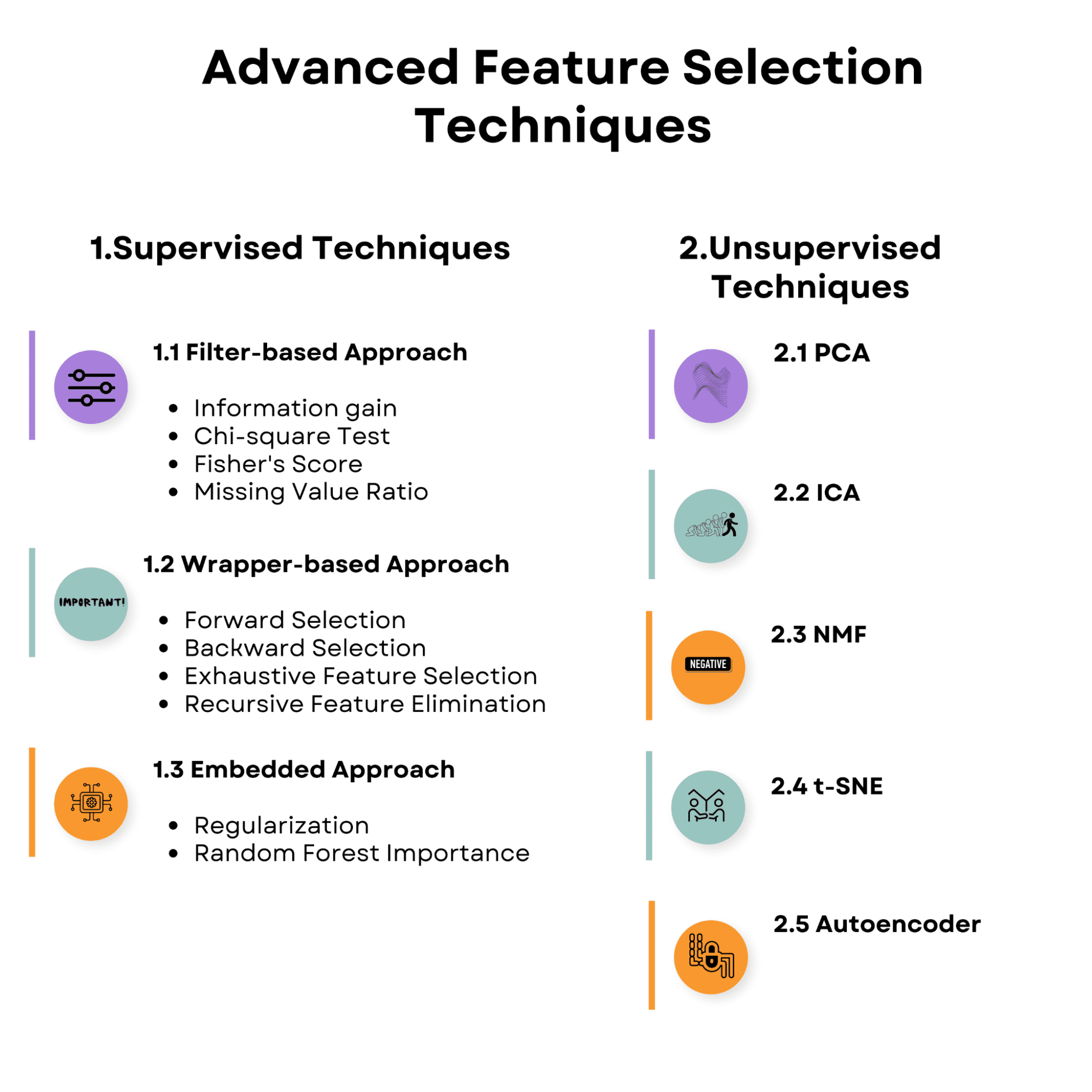
Take a look at the overview of the topics we’ll discuss in the article. Make yourself familiar with it, and let’s start with the supervised feature selection techniques.
Advanced Feature Selection Techniques for Machine Learning Models
Image by Author 1. Supervised Feature Selection Techniques

Feature selection strategies in supervised learning aim to discover the most relevant features for predicting the target variable by using the relationship between the input features and the target variable. These strategies might help improve model performance, reduce overfitting, and lower the computational cost of training the model.

Here’s the overview of the supervised feature selection techniques we’ll talk about.
Advanced Feature Selection Techniques for Machine Learning Models
Image by Author

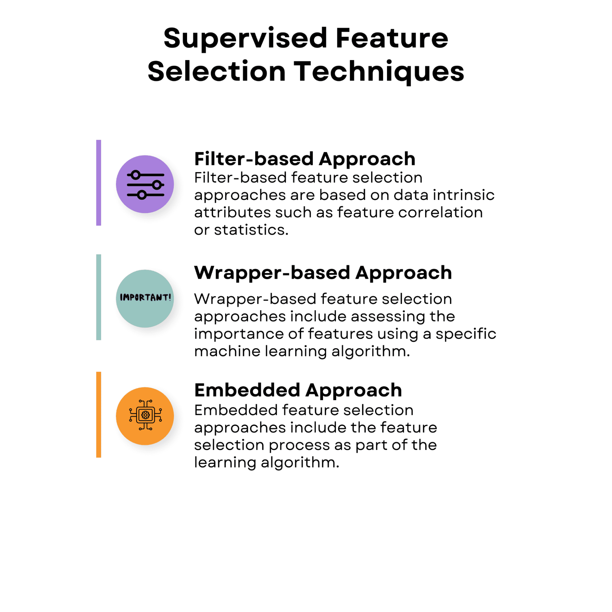
1.1 Filter-Based Approach

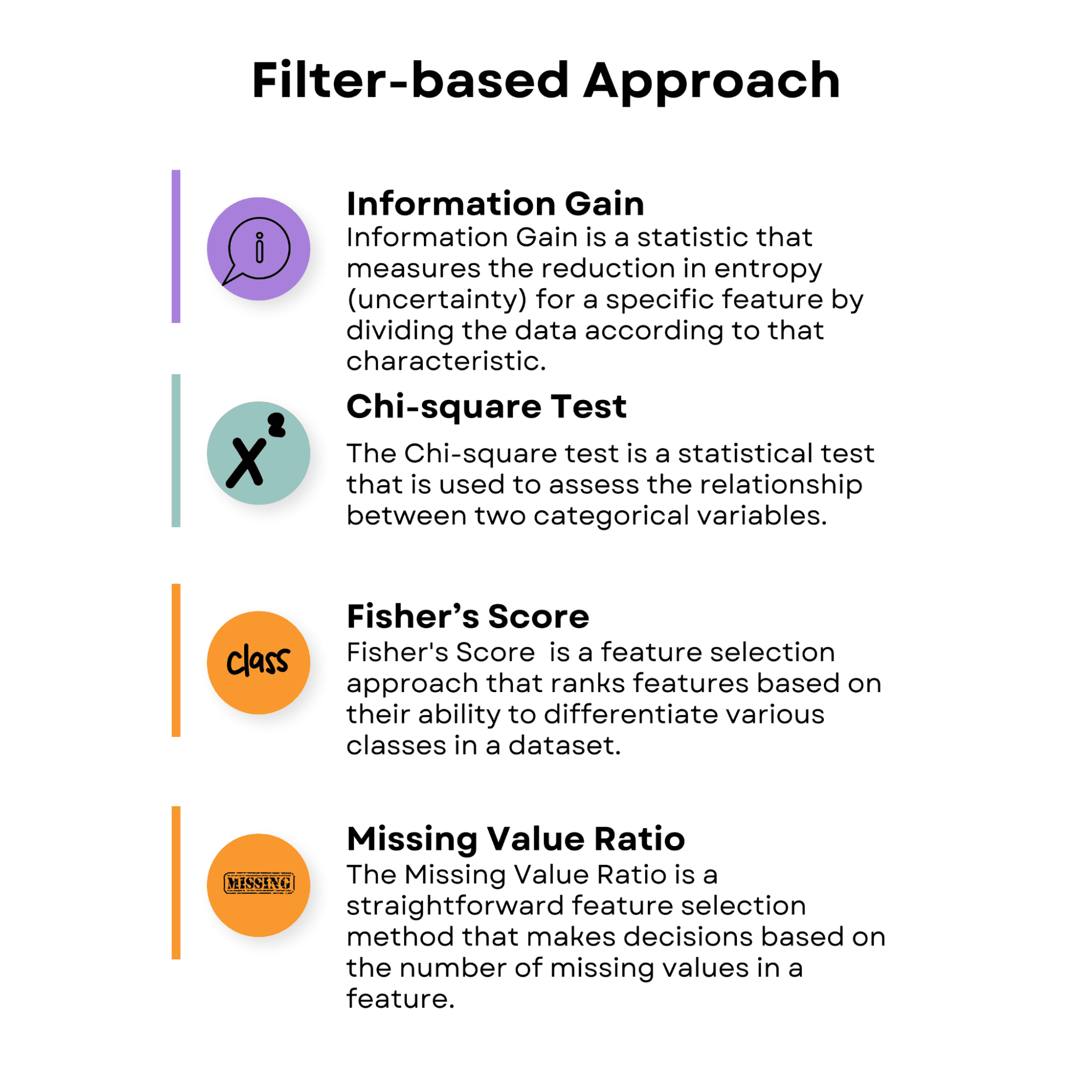
Filter-based feature selection approaches are based on data intrinsic attributes such as feature correlation or statistics. These approaches assess the value of each characteristic alone or in pairs without taking into account the performance of a particular learning algorithm.

Filter-based approaches are computationally efficient and may be used with a variety of learning algorithms. However, because they do not account for the interaction between the features and the learning method, they may not always capture the ideal feature subset for a certain algorithm.

Take a look at the overview of the filter-based approaches, and then we’ll discuss each.
Advanced Feature Selection Techniques for Machine Learning Models
Image by Author

Information Gain

Information Gain is a statistic that measures the reduction in entropy (uncertainty) for a specific feature by dividing the data according to that characteristic. It is often used in decision tree algorithms and also has useful features. The higher a feature's information gain, the more useful it is for decision-making.

Now, let’s apply information gain by using a prebuilt diabetes dataset.

The diabetes dataset contains physiological features related to predicting the progression of diabetes.

  • age: Age in years
  • sex: Gender (1 = male, 0 = female)
  • BMI: Body mass index, calculated as weight in kilograms divided by the square of height in meters
  • bp: Average blood pressure (mm Hg)
  • s1, s2, s3, s4, s5, s6: Blood serum measurements of six different blood chemicals (including glucose),

The following code demonstrates how to apply the Information Gain method. This code uses the diabetes dataset from the sklearn library as an example.

import numpy as np  import matplotlib.pyplot as plt  from sklearn.datasets import load_diabetes  from sklearn.feature_selection import mutual_info_regression    # Load the diabetes dataset  data = load_diabetes()    # Split the dataset into features and target  X = data.data  y = data.target

The primary objective of this code is to calculate feature importance scores based on Information Gain, which helps identify the most relevant features for the predictive model. By determining these scores, you can make informed decisions about which features to include or exclude from your analysis, ultimately leading to improved model performance, reduced overfitting, and faster training times.

To achieve this, this code calculates Information Gain scores for each feature in the dataset and stores them in a dictionary.

import numpy as np  import matplotlib.pyplot as plt  from sklearn.datasets import load_diabetes  from sklearn.feature_selection import mutual_info_regression    # Load the diabetes dataset  data = load_diabetes()    # Split the dataset into features and target  X = data.data  y = data.target    # Apply Information Gain  ig = mutual_info_regression(X, y)    # Create a dictionary of feature importance scores  feature_scores = {}  for i in range(len(data.feature_names)):      feature_scores[data.feature_names[i]] = ig[i]  

The features are then sorted in descending order according to their scores.

# Sort the features by importance score in descending order  sorted_features = sorted(feature_scores.items(), key=lambda x: x[1], reverse=True)    # Print the feature importance scores and the sorted features  for feature, score in sorted_features:      print('Feature:', feature, 'Score:', score)  

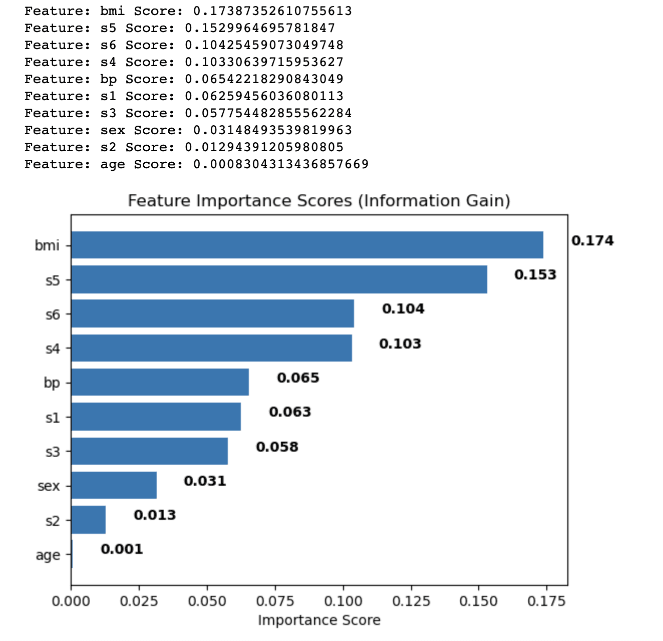
We will visualize the sorted feature importance scores as a horizontal bar chart, allowing you to easily compare the relevance of different features for the given task.

This visualization is particularly helpful when deciding which features to retain or discard while building a machine-learning model.

# Plot a horizontal bar chart of the feature importance scores  fig, ax = plt.subplots()  y_pos = np.arange(len(sorted_features))  ax.barh(y_pos, [score for feature, score in sorted_features], align="center")  ax.set_yticks(y_pos)  ax.set_yticklabels([feature for feature, score in sorted_features])  ax.invert_yaxis()  # Labels read top-to-bottom  ax.set_xlabel("Importance Score")  ax.set_title("Feature Importance Scores (Information Gain)")    # Add importance scores as labels on the horizontal bar chart  for i, v in enumerate([score for feature, score in sorted_features]):      ax.text(v + 0.01, i, str(round(v, 3)), color="black", fontweight="bold")  plt.show()  

Let’s see the whole code.

import numpy as np  import matplotlib.pyplot as plt  from sklearn.datasets import load_diabetes  from sklearn.feature_selection import mutual_info_regression    # Load the diabetes dataset  data = load_diabetes()    # Split the dataset into features and target  X = data.data  y = data.target    # Apply Information Gain  ig = mutual_info_regression(X, y)    # Create a dictionary of feature importance scores  feature_scores = {}  for i in range(len(data.feature_names)):      feature_scores[data.feature_names[i]] = ig[i]  # Sort the features by importance score in descending order  sorted_features = sorted(feature_scores.items(), key=lambda x: x[1], reverse=True)    # Print the feature importance scores and the sorted features  for feature, score in sorted_features:      print("Feature:", feature, "Score:", score)  # Plot a horizontal bar chart of the feature importance scores  fig, ax = plt.subplots()  y_pos = np.arange(len(sorted_features))  ax.barh(y_pos, [score for feature, score in sorted_features], align="center")  ax.set_yticks(y_pos)  ax.set_yticklabels([feature for feature, score in sorted_features])  ax.invert_yaxis()  # Labels read top-to-bottom  ax.set_xlabel("Importance Score")  ax.set_title("Feature Importance Scores (Information Gain)")    # Add importance scores as labels on the horizontal bar chart  for i, v in enumerate([score for feature, score in sorted_features]):      ax.text(v + 0.01, i, str(round(v, 3)), color="black", fontweight="bold")  plt.show()  

Here is the output.
Advanced Feature Selection Techniques for Machine Learning Models

The output shows the feature importance scores calculated using the Information Gain method for each feature in the diabetes dataset. The features are sorted in descending order based on their scores, which indicate their relative importance in predicting the target variable.

The results are as follows:

  • Body mass index (bmi) has the highest importance score (0.174), indicating that it has the most significant influence on the target variable in the diabetes dataset.
  • Serum measurement 5 (s5) follows with a score of 0.153, making it the second most important feature.
  • Serum measurement 6 (s6), serum measurement 4 (s4), and blood pressure (bp) have moderate importance scores, ranging from 0.104 to 0.065.
  • The remaining features, such as serum measurements 1, 2, and 3 (s1, s2, s3), sex, and age, have relatively lower importance scores, indicating that they contribute less to the predictive power of the model.

By analyzing these feature importance scores, you can decide which features to include or exclude from your analysis to improve the performance of your machine learning model. In this case, you might consider retaining features with higher importance scores, such as bmi and s5, while potentially removing or further investigating features with lower scores, such as age and s2.

Chi-square Test

The Chi-square test is a statistical test used to assess the relationship between two categorical variables. It is used in feature selection to analyze the relationship between a categorical feature and the target variable. A greater Chi-square score shows a stronger link between the feature and the target, showing that the feature is more important for the classification job.

While the Chi-square test is a commonly used feature selection method, it is typically used for categorical data, where the features and target variables are discrete.

Fisher’s Score

Fisher's Discriminant Ratio, commonly known as Fisher's Score, is a feature selection approach that ranks features based on their ability to differentiate various classes in a dataset. It may be used for continuous features in a classification problem.

Fisher's Score is calculated as the ratio of between-class and within-class variance. A higher Fisher's Score implies the characteristic is more discriminative and valuable for classification.

To use Fisher's Score for feature selection, compute a score for each continuous feature and rank them according to their scores. The model considers features with a higher Fisher's Score more important.

Missing Value Ratio

The Missing Value Ratio is a straightforward feature selection method that makes decisions based on the number of missing values in a feature.

Features having a significant proportion of missing values may be uninformative and may harm the model's performance. You can filter out features with too many missing values by specifying a threshold for the acceptable missing value ratio.

To use the Missing Value Ratio for feature selection, follow these steps:

  1. Calculate the missing value ratio for each feature by dividing the number of missing values by the total number of instances in the dataset.
  2. Set a threshold for the acceptable missing value ratio (e.g., 0.8, meaning that a feature should have at most 80% of its values missing to be considered).
  3. Filter out features that have a missing value ratio above the threshold.

1.2 Wrapper-Based Approach

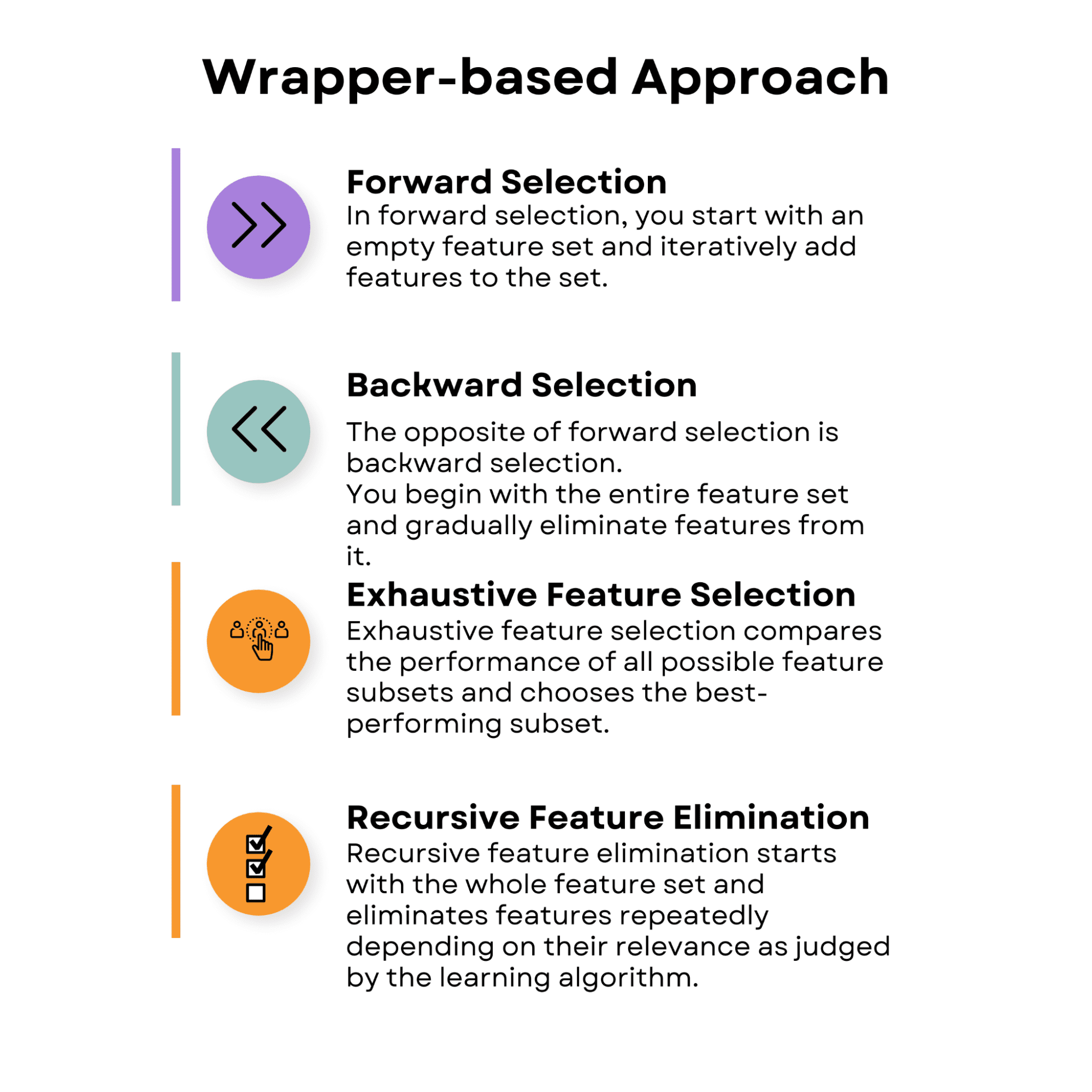
Wrapper-based feature selection approaches include assessing the importance of features using a specific machine learning algorithm. They seek the best subset of features by experimenting with various feature combinations and evaluating their performance with the selected method.

Because of the huge amount of available feature subsets, wrapper-based approaches can be computationally costly, especially when working with high-dimensional datasets.

However, they often outperform filter-based approaches because they consider the relationship between features and the learning algorithm.
Advanced Feature Selection Techniques for Machine Learning Models
Image by Author

Forward Selection

In forward selection, you start with an empty feature set and iteratively add features to the set. At each step, you evaluate the model's performance with the current feature set and the additional feature. The feature that results in the best performance improvement is added to the set.

The process continues until no significant improvement in performance is observed, or a predefined number of features is reached.

The following code demonstrates the application of forward selection, a wrapper-based supervised feature selection technique.

The example uses the breast cancer dataset from the sklearn library. The Breast Cancer dataset, also known as the Wisconsin Diagnostic Breast Cancer (WDBC) dataset, is a commonly used pre-built dataset for classification. And here, the main objective is building predictive models for diagnosing breast cancer as either malignant (cancerous) or benign (non-cancerous).

For the sake of our model, we will select a different number of features to see how performance changes accordingly, but first, let’s load the libraries, dataset, and variables.

import numpy as np  import pandas as pd  from sklearn.datasets import load_breast_cancer  from sklearn.linear_model import LogisticRegression  from sklearn.model_selection import train_test_split  from mlxtend.feature_selection import SequentialFeatureSelector as SFS    # Load the breast cancer dataset  data = load_breast_cancer()    # Split the dataset into features and target  X = data.data  y = data.target

The objective of the code is to identify an optimal subset of features for a logistic regression model using forward selection. This technique starts with an empty set of features and iteratively adds the features that improve the model's performance based on a specified evaluation metric. In this case, the metric used is accuracy.

The next part of the code employs the SequentialFeatureSelector from the mlxtend library to perform forward selection. It is configured with a logistic regression model, the desired number of features, and 5-fold cross-validation. The forward selection object is fitted to the training data, and the selected features are printed.

import numpy as np  import pandas as pd  from sklearn.datasets import load_breast_cancer  from sklearn.linear_model import LogisticRegression  from sklearn.model_selection import train_test_split  from mlxtend.feature_selection import SequentialFeatureSelector as SFS    # Load the breast cancer dataset  data = load_breast_cancer()    # Split the dataset into features and target  X = data.data  y = data.target    # Split the dataset into training and testing sets  X_train, X_test, y_train, y_test = train_test_split(X, y, test_size=0.3, random_state=0)    # Define the logistic regression model  model = LogisticRegression()    # Define the forward selection object  sfs = SFS(model,            k_features=5,            forward=True,            floating=False,            scoring='accuracy',            cv=5)    # Perform forward selection on the training set  sfs.fit(X_train, y_train)

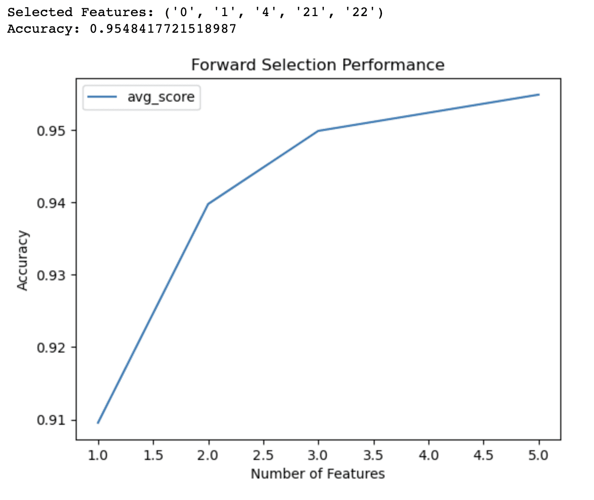
Additionally, we need to evaluate the performance of the selected features on the testing set and visualize the model's performance with different feature subsets in a line chart.

The chart will show the cross-validated accuracy as a function of the number of features, providing insights into the trade-off between model complexity and predictive performance.

By analyzing the output and the chart, you can determine the optimal number of features to include in your model, ultimately improving its performance and reducing overfitting.

# Print the selected features  print('Selected Features:', sfs.k_feature_names_)    # Evaluate the performance of the selected features on the testing set  accuracy = sfs.k_score_  print('Accuracy:', accuracy)    # Plot the performance of the model with different feature subsets  sfs_df = pd.DataFrame.from_dict(sfs.get_metric_dict()).T  sfs_df['avg_score'] = sfs_df['avg_score'].astype(float)  fig, ax = plt.subplots()  sfs_df.plot(kind='line', y='avg_score', ax=ax)  ax.set_xlabel('Number of Features')  ax.set_ylabel('Accuracy')  ax.set_title('Forward Selection Performance')  plt.show()

Here is the whole code.

import numpy as np  import pandas as pd  from sklearn.datasets import load_breast_cancer  from sklearn.linear_model import LogisticRegression  from sklearn.model_selection import train_test_split  from mlxtend.feature_selection import SequentialFeatureSelector as SFS    # Load the breast cancer dataset  data = load_breast_cancer()    # Split the dataset into features and target  X = data.data  y = data.target    # Split the dataset into training and testing sets  X_train, X_test, y_train, y_test = train_test_split(X, y, test_size=0.3, random_state=0)    # Define the logistic regression model  model = LogisticRegression()    # Define the forward selection object  sfs = SFS(model, k_features=5, forward=True, floating=False, scoring="accuracy", cv=5)    # Perform forward selection on the training set  sfs.fit(X_train, y_train)    # Print the selected features  print("Selected Features:", sfs.k_feature_names_)    # Evaluate the performance of the selected features on the testing set  accuracy = sfs.k_score_  print("Accuracy:", accuracy)    # Plot the performance of the model with different feature subsets  sfs_df = pd.DataFrame.from_dict(sfs.get_metric_dict()).T  sfs_df["avg_score"] = sfs_df["avg_score"].astype(float)  fig, ax = plt.subplots()  sfs_df.plot(kind="line", y="avg_score", ax=ax)  ax.set_xlabel("Number of Features")  ax.set_ylabel("Accuracy")  ax.set_title("Forward Selection Performance")  plt.show()  
Advanced Feature Selection Techniques for Machine Learning Models

The output of the forward selection code demonstrates that the algorithm has identified a subset of 5 features that yield the best accuracy (0.9548) for the logistic regression model on the breast cancer dataset. These selected features are identified by their indices: 0, 1, 4, 21, and 22.

The line graph provides additional insights into the performance of the model with different numbers of features. It shows that:

  • With just 1 feature, the model achieves an accuracy of around 91%.
  • Adding a second feature increases the accuracy to 94%.
  • With 3 features, the accuracy further improves to 95%.
  • Including 4 features pushes the accuracy slightly above 95%.

Beyond 4 features, the improvements in accuracy become less significant. This information can help you make informed decisions about the trade-offs between model complexity and predictive performance. Based on these results, you might decide to use only 3 or 4 features in your model to balance accuracy and simplicity.

Backward Selection

The opposite of forward selection is backward selection. You begin with the entire feature set and gradually eliminate features from it.

At each phase, you measure the model's performance with the current feature set minus the feature to be deleted.

The feature that causes the least amount of performance reduction gets eliminated from the set.

The procedure is repeated until there is no substantial increase in performance or a preset number of features is reached.

Backward and forward selections are categorized as a sequential feature selection; you can learn more here.

Exhaustive Feature Selection

Exhaustive feature selection compares the performance of all possible feature subsets and chooses the best-performing subset. This approach is computationally demanding, especially for large datasets, yet it ensures the best feature subset.

Recursive Feature Elimination

Recursive feature elimination starts with the whole feature set and eliminates features repeatedly depending on their relevance as judged by the learning algorithm. The least important feature is removed at each step, and the model is retrained. The method is repeated until a predetermined number of features are achieved.

1.3 Embedded Approach

Embedded feature selection approaches include the feature selection process as part of the learning algorithm.

This implies that throughout the training phase, the learning algorithm not only optimizes the model parameters but also picks the most important characteristics. Embedded methods can be more effective than wrapper methods since they do not require an external feature selection procedure.
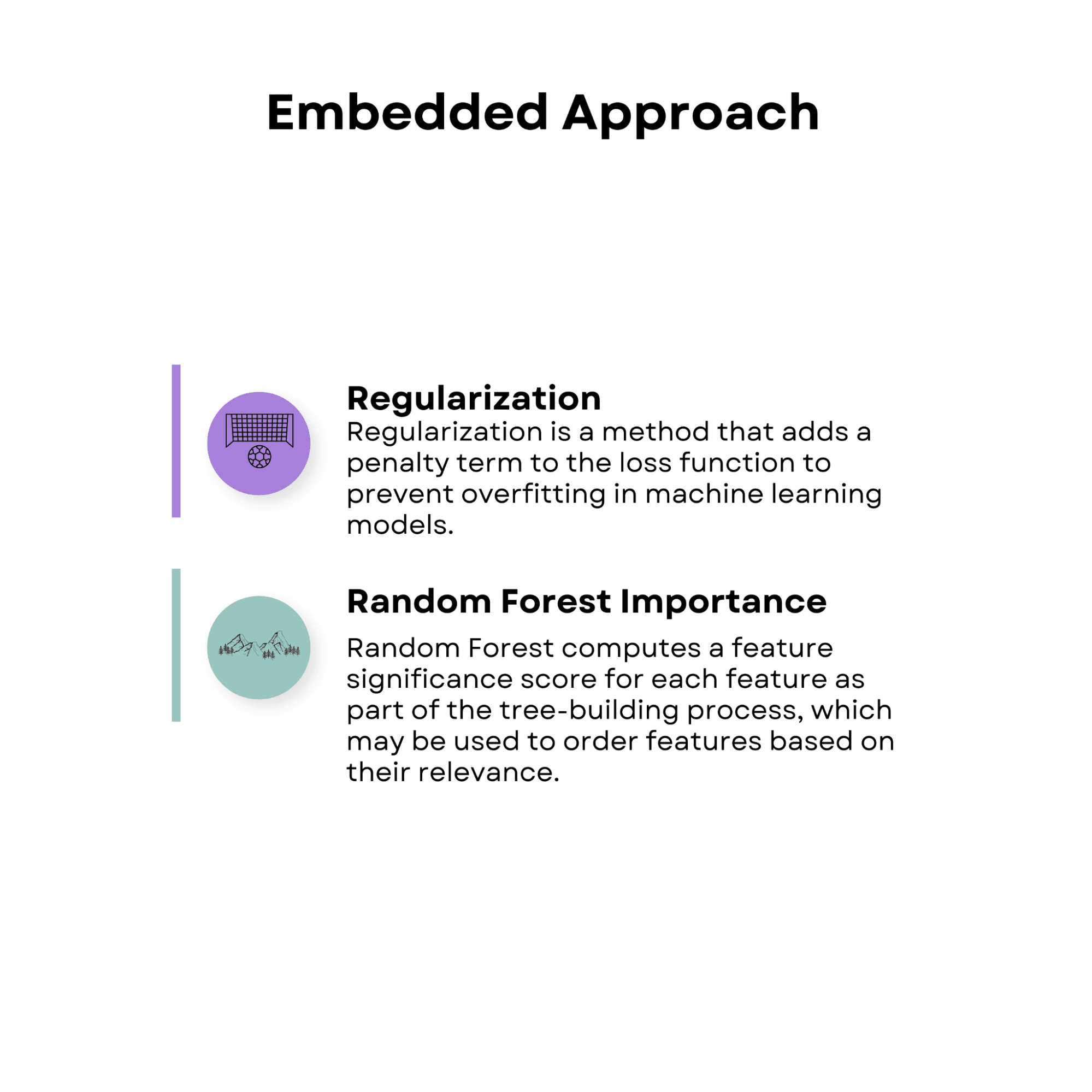
Advanced Feature Selection Techniques for Machine Learning Models
Image by Author

Regularization

Regularization is a method that adds a penalty term to the loss function to prevent overfitting in machine learning models.

Regularization methods, such as lasso (L1 regularization) and ridge (L2 regularization), can be used in conjunction with feature selection to decrease the coefficients of less significant features towards zero, thereby picking a subset of the most relevant features.

Random Forest Importance

Random forest is an ensemble learning approach that combines the predictions of several decision trees. Random forest computes a feature significance score for each feature as part of the tree-building process, which may be used to order features based on their relevance. The model considers features with higher significance ratings to be more significant.

If you want to learn more about the random forest, here is the article “Decision Tree and Random Forest Algorithm”, which also explains the decision tree algorithm too.

The following example uses the Covertype dataset, which includes information about different types of forest cover.

The aim of the Covertype dataset is to predict the forest cover type (the dominant tree species) within the Roosevelt National Forest of Northern Colorado.

The primary goal of the below code is to determine the importance of features using a random forest classifier. By evaluating the contribution of each feature to the overall classification performance, this method helps identify the most relevant features for building a predictive model.

import pandas as pd  import numpy as np  from sklearn.ensemble import RandomForestClassifier  from sklearn.model_selection import train_test_split  import matplotlib.pyplot as plt    # Load the Covertype dataset  data = pd.read_csv("https://archive.ics.uci.edu/ml/machine-learning-databases/covtype/covtype.data.gz", header=None)    # Assign column names  cols = ["Elevation", "Aspect", "Slope", "Horizontal_Distance_To_Hydrology",          "Vertical_Distance_To_Hydrology", "Horizontal_Distance_To_Roadways",          "Hillshade_9am", "Hillshade_Noon", "Hillshade_3pm",          "Horizontal_Distance_To_Fire_Points"] + ["Wilderness_Area_"+str(i) for i in range(1,5)] + ["Soil_Type_"+str(i) for i in range(1,41)] + ["Cover_Type"]    data.columns = cols

Then, we create a RandomForestClassifier object and fit it to the training data. It then extracts the feature importances from the trained model and sorts them in descending order. The top 10 features are selected based on their importance scores and displayed in a ranking.

# Split the dataset into train and test sets  X_train, X_test, y_train, y_test = train_test_split(X, y, test_size=0.3, random_state=42)    # Create a random forest classifier object  rfc = RandomForestClassifier(n_estimators=100, random_state=42)    # Fit the model to the training data  rfc.fit(X_train, y_train)    # Get feature importances from the trained model  importances = rfc.feature_importances_    # Sort the feature importances in descending order  indices = np.argsort(importances)[::-1]      # Select the top 10 features  num_features = 10  top_indices = indices[:num_features]  top_importances = importances[top_indices]      # Print the top 10 feature rankings  print("Top 10 feature rankings:")  for f in range(num_features):  # Use num_features instead of 10      print(f"{f+1}. {X_train.columns[indices[f]]}: {importances[indices[f]]}")

Additionally, the code visualizes the top 10 feature importances using a horizontal bar chart.

# Plot the top 10 feature importances in a horizontal bar chart  plt.barh(range(num_features), top_importances, align='center')  plt.yticks(range(num_features), X_train.columns[top_indices])  plt.xlabel("Feature Importance")  plt.ylabel("Feature")  plt.show()

This visualization allows for easy comparison of the importance scores and aids in making informed decisions about which features to include or exclude from your analysis.

By examining the output and the chart, you can select the most relevant features for your predictive model, which can help improve its performance, reduce overfitting, and accelerate training times.

Here is the whole code.

import pandas as pd  import numpy as np  from sklearn.ensemble import RandomForestClassifier  from sklearn.model_selection import train_test_split  import matplotlib.pyplot as plt    # Load the Covertype dataset  data = pd.read_csv(      "https://archive.ics.uci.edu/ml/machine-learning-databases/covtype/covtype.data.gz",      header=None,  )    # Assign column names  cols = (      [          "Elevation",          "Aspect",          "Slope",          "Horizontal_Distance_To_Hydrology",          "Vertical_Distance_To_Hydrology",          "Horizontal_Distance_To_Roadways",          "Hillshade_9am",          "Hillshade_Noon",          "Hillshade_3pm",          "Horizontal_Distance_To_Fire_Points",      ]      + ["Wilderness_Area_" + str(i) for i in range(1, 5)]      + ["Soil_Type_" + str(i) for i in range(1, 41)]      + ["Cover_Type"]  )    data.columns = cols    # Split the dataset into features and target  X = data.iloc[:, :-1]  y = data.iloc[:, -1]    # Split the dataset into train and test sets  X_train, X_test, y_train, y_test = train_test_split(      X, y, test_size=0.3, random_state=42  )    # Create a random forest classifier object  rfc = RandomForestClassifier(n_estimators=100, random_state=42)    # Fit the model to the training data  rfc.fit(X_train, y_train)    # Get feature importances from the trained model  importances = rfc.feature_importances_    # Sort the feature importances in descending order  indices = np.argsort(importances)[::-1]      # Select the top 10 features  num_features = 10  top_indices = indices[:num_features]  top_importances = importances[top_indices]      # Print the top 10 feature rankings  print("Top 10 feature rankings:")  for f in range(num_features):  # Use num_features instead of 10      print(f"{f+1}. {X_train.columns[indices[f]]}: {importances[indices[f]]}")  # Plot the top 10 feature importances in a horizontal bar chart  plt.barh(range(num_features), top_importances, align="center")  plt.yticks(range(num_features), X_train.columns[top_indices])  plt.xlabel("Feature Importance")  plt.ylabel("Feature")  plt.show()  

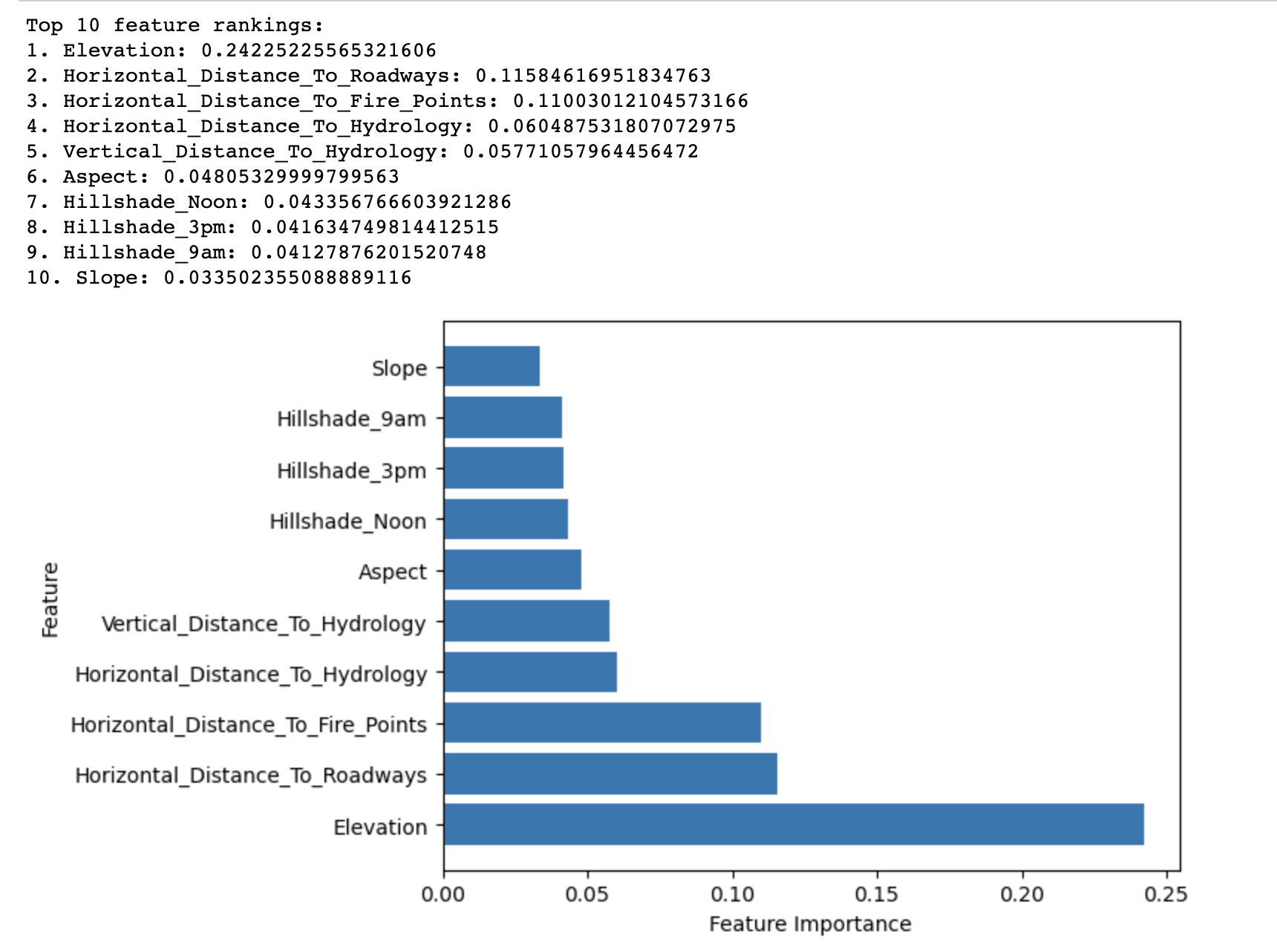
Here is the output.
Advanced Feature Selection Techniques for Machine Learning Models

The output of the Random Forest Importance method displays the top 10 features ranked by their importance in predicting the forest cover type in the Covertype dataset.

It reveals that Elevation has the highest importance score (0.2423) among all features in predicting the forest cover type. This suggests that elevation plays a critical role in determining the dominant tree species in the Roosevelt National Forest.

Other features with relatively high importance scores include Horizontal_Distance_To_Roadways (0.1158) and Horizontal_Distance_To_Fire_Points (0.1100). These indicate that proximity to roadways and fire ignition points also significantly impacts forest cover types.

The remaining features in the top 10 list have relatively lower importance scores, but they still contribute to the overall predictive performance of the model. These features mainly relate to hydrological factors, slope, aspect, and hillshade indices.

In summary, the results highlight the most important factors affecting the distribution of forest cover types in the Roosevelt National Forest, which can be used to build a more effective and efficient predictive model for forest cover type classification.

2. Unsupervised Feature Selection Techniques

When there is no target variable available, unsupervised feature selection approaches can be used in order to reduce the dimensionality of the dataset while keeping its underlying structure. These methods often include changing the initial feature space into a new lower-dimensional space in which the changed features capture the majority of the variation in the data.
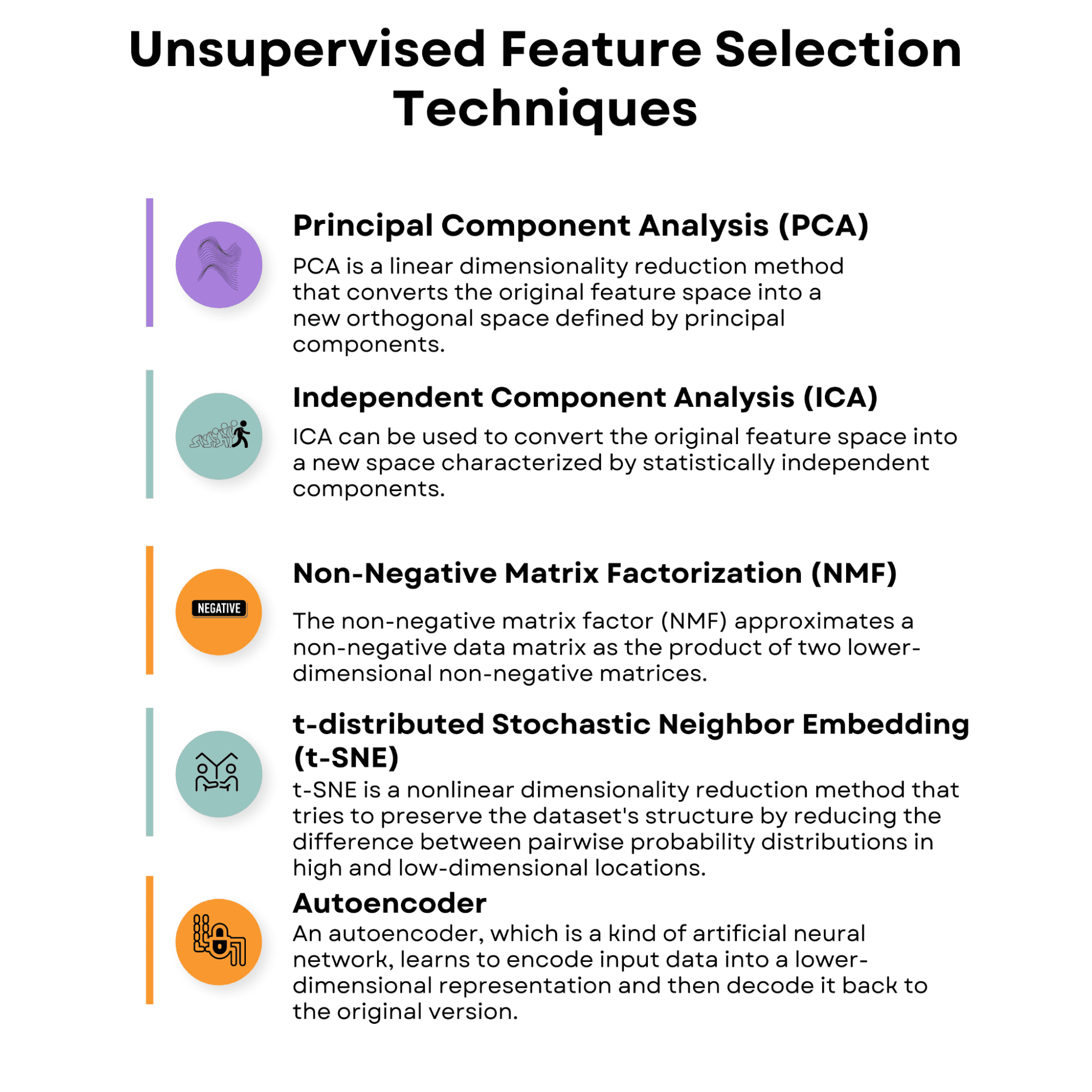
Advanced Feature Selection Techniques for Machine Learning Models
Image by Author

2.1 Principal Component Analysis (PCA)

PCA is a linear dimensionality reduction method that converts the original feature space into a new orthogonal space defined by principal components. These components are linear combinations of the original features chosen to capture the highest level of variance in the data.

PCA may be used to pick the top k principal components representing most of the variation, thus lowering the dataset's dimensionality.

To show you how this works in practice, we will work with the Wine dataset. This is a widely used dataset for classification and feature selection tasks in machine learning and consists of 178 samples, each representing a different wine originating from three different cultivars in the same region in Italy.

The goal of working with the Wine dataset is usually to build a predictive model that can accurately classify a wine sample into one of the three cultivars based on its chemical properties.

The following code demonstrates the application of Principal Component Analysis (PCA), an unsupervised feature selection technique, on the Wine dataset.

These components(principal components) capture the most variance in the data while minimizing the information loss.

The code starts by loading the Wine dataset, which consists of 13 features describing the chemical properties of different wine samples.

import numpy as np  import pandas as pd  import matplotlib.pyplot as plt  from sklearn.datasets import load_wine  from sklearn.decomposition import PCA  from sklearn.preprocessing import StandardScaler    # Load the Wine dataset  wine = load_wine()  X = wine.data  y = wine.target  feature_names = wine.feature_names

These features are then standardized using the StandardScaler to ensure that PCA is not affected by varying scales of the input features.

# Standardize the features  scaler = StandardScaler()  X_scaled = scaler.fit_transform(X)

Next, PCA is performed on the standardized data using the PCA class from the sklearn.decomposition module.

# Perform PCA  pca = PCA()  X_pca = pca.fit_transform(X_scaled)

The explained variance ratio for each principal component is calculated, indicating the proportion of the total variance in the data that each component explains.

# Calculate the explained variance ratio  explained_variance_ratio = pca.explained_variance_ratio_

Finally, two plots are generated to visualize the explained variance ratio and the cumulative explained variance by the principal components.

The first plot shows the explained variance ratio for each individual principal component, while the second plot illustrates how the cumulative explained variance increases as more principal components are included.

These plots help determine the optimal number of principal components to use in the model, balancing the trade-off between dimensionality reduction and information retention.

# Create a 2x1 grid of subplots  fig, (ax1, ax2) = plt.subplots(nrows=1, ncols=2, figsize=(16, 8))    # Plot the explained variance ratio in the first subplot  ax1.bar(range(1, len(explained_variance_ratio) + 1), explained_variance_ratio)  ax1.set_xlabel('Principal Component')  ax1.set_ylabel('Explained Variance Ratio')  ax1.set_title('Explained Variance Ratio by Principal Component')    # Calculate the cumulative explained variance  cumulative_explained_variance = np.cumsum(explained_variance_ratio)    # Plot the cumulative explained variance in the second subplot  ax2.plot(range(1, len(cumulative_explained_variance) + 1), cumulative_explained_variance, marker='o')  ax2.set_xlabel('Number of Principal Components')  ax2.set_ylabel('Cumulative Explained Variance')  ax2.set_title('Cumulative Explained Variance by Principal Components')    # Display the figure  plt.tight_layout()  plt.show()  

Let’s see the whole code.

import numpy as np  import pandas as pd  import matplotlib.pyplot as plt  from sklearn.datasets import load_wine  from sklearn.decomposition import PCA  from sklearn.preprocessing import StandardScaler    # Load the Wine dataset  wine = load_wine()  X = wine.data  y = wine.target  feature_names = wine.feature_names    # Standardize the features  scaler = StandardScaler()  X_scaled = scaler.fit_transform(X)    # Perform PCA  pca = PCA()  X_pca = pca.fit_transform(X_scaled)    # Calculate the explained variance ratio  explained_variance_ratio = pca.explained_variance_ratio_    # Create a 2x1 grid of subplots  fig, (ax1, ax2) = plt.subplots(nrows=1, ncols=2, figsize=(16, 8))    # Plot the explained variance ratio in the first subplot  ax1.bar(range(1, len(explained_variance_ratio) + 1), explained_variance_ratio)  ax1.set_xlabel("Principal Component")  ax1.set_ylabel("Explained Variance Ratio")  ax1.set_title("Explained Variance Ratio by Principal Component")    # Calculate the cumulative explained variance  cumulative_explained_variance = np.cumsum(explained_variance_ratio)    # Plot the cumulative explained variance in the second subplot  ax2.plot(      range(1, len(cumulative_explained_variance) + 1),      cumulative_explained_variance,      marker="o",  )  ax2.set_xlabel("Number of Principal Components")  ax2.set_ylabel("Cumulative Explained Variance")  ax2.set_title("Cumulative Explained Variance by Principal Components")    # Display the figure  plt.tight_layout()  plt.show()  

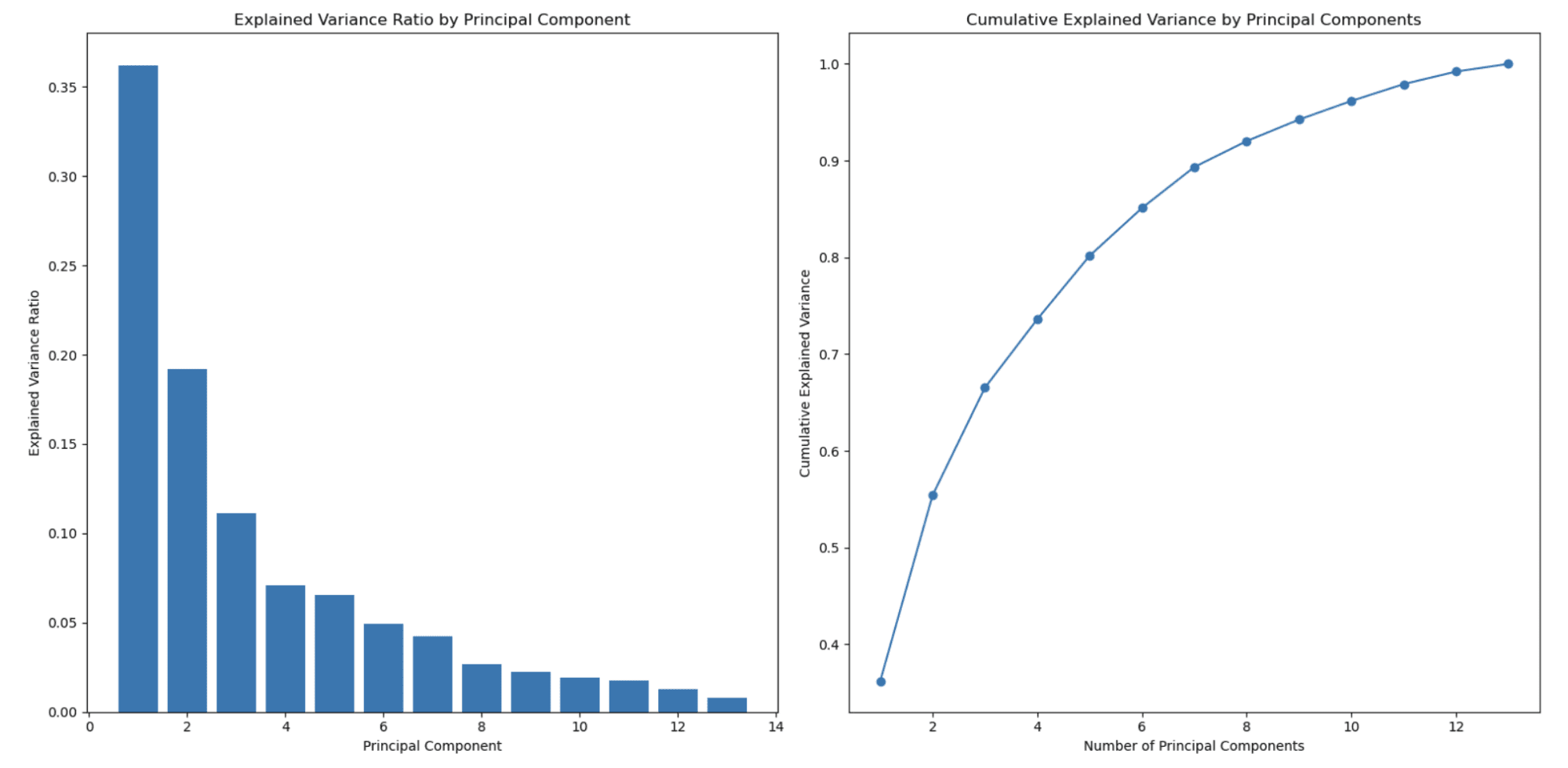
Here is the output.
Advanced Feature Selection Techniques for Machine Learning Models

The graph on the left shows that the explained variance ratio decreases as the number of principal components increases. This is a typical behavior observed in PCA because principal components are ordered by the amount of variance they explain.

The first principal component (feature) captures the highest variance, the second principal component captures the second highest amount, and so on. As a result, the explained variance ratio decreases with each subsequent principal component.

This is one of the main reasons PCA is used for dimensionality reduction.

The second graph on the right shows the cumulative explained variance and helps you determine how many principal components (features) to select to represent the percentage of your data. The x-axis represents the number of principal components, and the y-axis shows the cumulative explained variance. As you move along the x-axis, you can see how much of the total variance is retained when you include that many principal components.

In this example, you can see that selecting around 3 or 4 principal components already captures more than 80% of the total variance, and around 8 principal components capture over 90% of the total variance.

You can choose the number of principal components based on your desired trade-off between dimensionality reduction and the variance you want to retain.

In this example, we did use Sci-kit to learn to apply PCA, and here you can find the official document.

2.2 Independent Component Analysis (ICA)

ICA is a method for dividing a multidimensional signal into its components.

In the context of feature selection, ICA can be used to convert the original feature space into a new space characterized by statistically independent components. You may decrease the dimensionality of the dataset while keeping the underlying structure by picking the top k independent components.

2.3 Non-Negative Matrix Factorization (NMF)

The non-negative matrix factor (NMF) is a dimensionality reduction approach that approximates a non-negative data matrix as the product of two lower-dimensional non-negative matrices.

NMF can be used in the context of feature selection to extract a new set of basic features that capture the important structure of the original data. You may minimize the dimensionality of the dataset while maintaining the non-negativity limitation by picking the top k basis features.

2.4 t-distributed Stochastic Neighbor Embedding (t-SNE)

t-SNE is a nonlinear dimensionality reduction method that tries to preserve the dataset's structure by reducing the difference between pairwise probability distributions in high and low-dimensional locations.

t-SNE may be applied in feature selection to project the original feature space into a lower-dimensional space that maintains the structure of the data, allowing enhanced visualization and evaluation.

You can find more information about both unsupervised algorithms and t-SNE here “Unsupervised Learning Algorithms”.

2.5 Autoencoder

An autoencoder, a kind of artificial neural network, learns to encode input data into a lower-dimensional representation and then decode it back to the original version. The autoencoder's lower-dimensional representation can be used to produce another set of features that capture the underlying structure of the original data.

Final Words

In conclusion, feature selection is vital in machine learning. It helps reduce the data's dimensionality, minimize the risk of overfitting, and improve the model's overall performance. Choosing the right feature selection method depends on the specific problem, dataset, and modeling requirements.

This article covered a wide range of feature selection techniques, including supervised and unsupervised methods.

Supervised techniques, such as filter-based, wrapper-based, and embedded approaches, use the relationship between features and the target variable to identify the most important features.

Unsupervised techniques, like PCA, ICA, NMF, t-SNE, and autoencoders, focus on the intrinsic structure of the data to reduce dimensionality without considering the target variable.

When selecting the appropriate feature selection method for your model, it's vital to consider the characteristics of your data, the underlying assumptions of each technique, and the computational complexity involved.

By carefully selecting and applying the right feature selection technique, you can significantly enhance the performance, leading to better insights and decision-making.
Nate Rosidi is a data scientist and in product strategy. He's also an adjunct professor teaching analytics, and is the founder of StrataScratch, a platform helping data scientists prepare for their interviews with real interview questions from top companies. Connect with him on Twitter: StrataScratch or LinkedIn.

More On This Topic

  • Alternative Feature Selection Methods in Machine Learning
  • Feature Selection – All You Ever Wanted To Know
  • Why Automated Feature Selection Has Its Risks
  • Feature Selection: Where Science Meets Art
  • This Data Visualization is the First Step for Effective Feature Selection
  • Be Wary of Automated Feature Selection — Chi Square Test of Independence…

Singapore creates digital blueprint for generative AI and autonomous systems

Singapore financial district

Singapore has laid out a years-long roadmap it believes will ensure its digital infrastructure is ready to tap emerging technologies, such as generative artificial intelligence (AI), autonomous systems, and immersive multi-party interactions.

The Digital Connectivity Blueprint maps out key priorities for the country's infrastructure over the next 10 years and serves as a foundation on which it can realize better opportunities, said Minister for Communications and Information Josephine Teo.

Also: Today's AI boom will amplify social problems if we don't act now, says AI ethicist

The blueprint encompasses physical infrastructures, including broadband, mobile networks and data centers, as well as "digital utilities" to facilitate secure and seamless cross-border transactions. These transactions include e-payments and invoicing, data exchanges, document authentication, and identity verification, said Teo.

She added that the blueprint will place Singapore in a better position to embrace opportunities from emerging technology trends, such as generative AI and autonomous vehicles.

The roadmap will require significant resources, she noted, pointing to submarine cables and data centers as two big-ticket items that will drive some SG$20 billion ($14.78 billion) in investments. Of this, SG$10 billion to SG$12 billion is expected to go toward building new green data centers, Teo said, adding that the private sector will fund most of the investments.

Also: How to make tech more sustainable: Five ways to make it happen

The Digital Connectivity Blueprint outlines plans to build 10Gbps nationwide connectivity in the next five years and provide capacity to double subsea cable landings within the next decade.

"We will intensify the use of space and landing resources available, so operators can expand and further diversify the network of submarine cables," said the Infocomm Media Development Authority (IMDA), which developed the roadmap with the Ministry of Communications and Information. Efforts here will boost digital connectivity between Singapore, Southeast Asia, and other regions, IMDA said.

The government agency added that spectrum will be allocated to enable faster Wi-Fi networks and standalone 5G networks to further improve their performance and support business adoption. "We envision a future where smooth 'handover' between different modes of connectivity also enables seamless movement between outdoor and indoor environments, paving the way for game-changing innovations, such as in logistics," the agency said.

Also: AI will change the role of developers forever. Here's why that's good news

Some 98% of households in Singapore currently have broadband access, typically at 1Gbps speeds. The goal is to bump this up to 10Gbps over the next five years, as Wi-Fi 6E and 5G standalone networks are rolled out. Infrastructure upgrades to achieve these speeds will begin in mid-2024, according to IMDA.

There also will be initiatives in other nascent areas, such as quantum computing, where Singapore will aim to be quantum safe within the next 10 years. The country's dense urban environment and pervasive fiber network present an advantage in implementing quantum-safe communications, IMDA said.

The government agency said plans are in place to pilot quantum-safe networks and quantum-as-a-service applications for commercial customers. "Known as the National Quantum Safe Network Plus (NQSN+), this will allow us to test, innovate and push the boundaries on both technical and commercial deployments," it said.

Launch of innovation center with AWS

IMDA on Monday also announced its partnership with Amazon Web Services (AWS) through the launch of a joint innovation center. Pitched as a launchpad for businesses and startups in Southeast Asia, the new site houses various specialized labs, including 5G as well as augmented and virtual reality. It also has usability-testing facilities.

Located at IMDA's own innovation hub Pixel, the innovation center will provide "exclusive access" to the latest technologies and methodologies for successful deployment, the Singapore agency said. More than 200 AWS technology offerings are available for experimentation, alongside project-based consultation with experts from IMDA and AWS.

Also: Low-code platforms mean anyone can be a developer

The new innovation center will also provide connections to both IMDA's and AWS' network of startups and organizations across Southeast Asia, and the U.S. cloud vendor's partners.

Companies can use the center to develop proof-of-concepts in a sandbox environment. The innovation center will showcase tech offerings built on AWS and from startups participating in IMDA's various programs, including accreditation schemes.

How to use Bing Image Creator (and why it’s better than DALL-E 2)

Bing Image Creator

A photo generated with the Bing Image Creator using the prompt "a photo of a robot taking a picture with a DSLR camera in a studio".

As the use of different artificial intelligence tools has exploded in recent months, we've seen the development of generative AI sprouting in the most unlikely places. It all began with the preview launch of ChatGPT last fall, a conversational AI chatbot from OpenAI that has amazed users with its natural tone, ease of accessibility, and usefulness.

How to use: Midjourney | Craiyon AI | DALL-E 2 | Stable Diffusion

Since then, both Google and Microsoft have released their own AI chatbots with Bard and Bing Chat, respectively, even though the AI craze hasn't been without its security, ethical, and economic concerns. Microsoft also released an AI image creator within Bing, using a more advanced version of DALL-E 2, another one of OpenAI's projects.

Similar to using ChatGPT, the DALL-E 2 image generator is accessed by logging into OpenAI's website, where users can then enter a prompt in a text area and wait while it creates an image using AI.

There are some key differences between how Bing Image Creator and the original DALL-E 2 work, however, and we'll explore some of those as we go along.

Also: The best AI art generators to try

First, let's dive into learning how to use the new Bing Image Creator.

How to use the new Bing Image Creator

Image created by Bing Image Creator using the prompt "photo of a lazy zebra in a room with navy walls and gold curtains".

What you need: Using the Bing Image Creator only requires a Microsoft account and access to Bing.com, no need for a DALL-E 2 or OpenAI account. The Bing Image Creator can be accessed via Bing Chat or by going to Bing.com/Create. We'll cover the former option below in the FAQ and the latter in detail here.

On the homepage for the Bing Image Creator, click on Join & Create.

Enter your prompt in the text area.

For this prompt, I'm going to request the following: "photo of a swan laying in a royal living room with gold accents". Then I'm going to click on Create and wait for my images to be generated.

The Bing Image Creator preview results created with the prompt I entered (highlighted at the top).

This was my favorite photo of the four.

FAQ

Can I create images using the new Bing Chat?

There are two ways to use the Bing Image Creator. You can generate images by going to Bing.com/Create, as detailed above, or you can create images right from Bing Chat.

I asked Bing Chat to create a photo of a monkey on a Vespa and it didn't disappoint.

Here's how you can ask the new Bing to create an image right from the chat window:

  1. Open Microsoft Edge
  2. Go to Bing.com
  3. Click on Chat
  4. Write your prompt, it can begin with a phrase like "create an image" or "generate a photo", but it's not necessary. Bing Chat typically recognizes your intent.

Also: How to use the new Bing (and how it's different from ChatGPT)

Bing Chat can create images in any conversation style, whether it's set to Creative, Balanced, or Precise.

One of the pros to using Bing Chat to generate images is that you can ask follow-up questions to have Bing adjust the image, like the example above shows. Bing proposes questions like, "Can you make the monkey wear a hat?" and "Change the color of the Vespa to blue".

How do you write prompts to create images using AI?

The more specific you are in your prompts, the better; think of the prompt as a detailed description of the image you have in mind. Include adjectives, nouns, and verbs to describe the image and what the subject is doing — even styles are encouraged. If you say, "create a photo of…" you'll get a different result than if you say create a cartoon, a painting, or a 3D render; so the image style is important.

This is the best way to build a successful Bing Image Creator prompt.

Here's how Bing's Image Creator recommends you format your prompts: Adjective + Noun + Verb + Style.

Also: I've tested a lot of AI tools for work. These are my 5 favorite so far

In this case, that would be "Fuzzy creature wearing sunglasses, digital art."

You can use different terms to describe the style, as well, like impressionism, cubism, abstract, etc.

Do I own AI-generated images?

The latest line from the United States Copyright Office (USCO) is that AI-generated images are not protected under current copyright laws because they are not the product of human authorship.

AI image generators have created controversy as they're AI bots trained on images found online, images that have been created by someone else. While the art you created using an image creator tool is unique, it's created with influences of millions of artists on the internet.

Also: The White House seeks your opinion on ChatGPT and AI tools for safety policy

This ruling is subject to change as the USCO holds listening sessions throughout 2023 to explore the subject more deeply and make necessary changes.

Is Bing Image Creator free?

Bing's Image Creator is free at this time, though you can pay for more boosts if you run out. Boosts are like credits, where each prompt you give it to create an image will cost you one of your boosts. Users used to get 25 when they'd first start using the Image Creator, but it has since increased to 100.

Also: ChatGPT vs. Bing Chat: Which AI chatbot should you use?

Once you run out of boosts, the Bing Image Creator will take longer to generate images after it's given a prompt. Instead of 10-30 seconds, it can take up to five minutes.

Microsoft was refilling boosts on a weekly basis, but has now switched to doing so daily. Users also have the option of redeeming Microsoft rewards in exchange for more boosts.

Is Bing Image Creator the same as DALL-E 2?

DALL-E 2 and the Bing Image Creator are not the same. Like with GPT-4 in Bing Chat, Microsoft is incorporating a more advanced version of the AI art generator into its image creator.

Though the same prompt won't render the same results twice, you can see the comparison of images created with both DALL-E 2 (left) and Bing Image Creator (right).

Also: Generative AI can save marketing pros 5 hours per week, according to research

Beyond artistic differences, the Bing images boast better attention to detail and vibrancy than the DALL-E 2 images.

Is there a waitlist to use the Bing Image Creator?

There is no waitlist to use the Bing Image Creator at this time. All you have to do is log in to the website with your Microsoft account and you'll have access to it.

More on AI tools

AutoGPT: Everything You Need To Know About This NLP-Based Autonomous AI Agent

Featured Blog Image-AutoGPT: Everything You Need To Know About This NLP-Based Autonomous AI Agent

The emergence of AutoGPT – a groundbreaking open-source application developed using the state-of-the-art GPT-3.5 & GPT-4 large language models (LLMs), has generated significant excitement within the Artificial Intelligence (AI) community.

AutoGPT is an advanced autonomous AI agent developed by Toran Bruce Richards, designed to generate prompts for the underlying language model to execute tasks automatically without human intervention based on a predefined goal. It can break down complex goals and generate contextually relevant responses.

Let’s give a comprehensive overview of AutoGPT and discuss its fundamental features.

How Does AutoGPT Work?

AutoGPT can gather task-related information from the internet using a combination of advanced methods for Natural Language Processing (NLP) and autonomous AI agents. Unlike regular LLMs that need well-defined input prompts from humans, AutoGPT generates prompts to complete all the subtasks of a defined goal. Hence, users don’t have to craft follow-up responses for the model’s outcome.

AutoGPT depends on four key aspects:

  • Model Architecture: AutoGPT is built on top of robust transformer-based GPT-4 and GPT-3.5 LLMs developed by OpenAI. These models aid in thought and reasoning to complete tasks.
  • Autonomous Iterations: AutoGPT AI agents evaluate task progress, build on prior outcomes, and utilize history to achieve a goal.
  • Memory Management: AutoGPT can maintain context and make smarter judgments due to effective long-term and short-term memory management using an in-memory datastore like Redis.
  • Multifunctionality: AutoGPT distinguishes itself from earlier AI developments due to its multifunctional capabilities, including internet browsing, data retrieval, text generation, file storage and summarization, image generation, and extensibility using plugins.

3 Major Benefits of AutoGPT & How It Supercharges NLP?

AutoGPT brings the following benefits to its users by enhancing the efficiency of language-related tasks:

1. Real-Time Insights

Traditional NLP models are trained on large but limited data since they cannot access the web to fetch the latest data. Using AutoGPT, users can get real-time insights for any task as it can gather up-to-date information from popular websites and platforms. It can help businesses look at the latest trends and make informed data-driven decisions quickly.

2. Memory Management

One of the challenges that LLMs face is their ability to retain previous sequences of information due to memory limitation. AutoGPT can save and retrieve data from past exchanges using a memory cache. It can either use a local cache that saves information in JSON format or leverage external data stores like Redis. Hence, robust memory management improves the model's contextual awareness and enables it to deliver more tailored responses.

3. Enhanced Productivity

AutoGPT frees up significant time and resources by automating repetitive procedures, enabling people and organizations to concentrate on more difficult and strategic projects. Without human assistance, it can generate text, respond to inquiries, conduct extensive research, and roleplay specialized designations like a marketing manager or copywriter, based on a user-defined goal.

Top 5 Use Cases of AutoGPT

AutoGPT demonstrates the potential of autonomous AI systems that can revolutionize numerous sectors by enabling seamless human-AI interactions. It has a wide range of use uses, such as:

1. Creative Storytelling & Content Writing

AutoGPT's autonomous text-generation capabilities can be used for storytelling and creative writing. It can help authors, screenwriters, copywriters, and marketers in creating plots, writing character dialogues, fresh ad copies, and blogs.

2. Data Analysis, Visualisation, & Development

AutoGPT can extract important insights from huge datasets. It can automatically surf the web to set up a development environment, install relevant programming libraries, and write code (or boilerplate code at least) to analyze datasets based on user-defined goals. It can understand intricate data relationships and patterns to detect trends, make predictions, and create intuitive visuals autonomously. As a result, businesses, developers, and researchers can make informed decisions.

3. Text to Speech

AutoGPT can transform any text into realistic speech autonomously. It can integrate with ElevanLabs to leverage voice technologies such as speech synthesis, voice design, and premade lifelike voices. As a result, companies can build various tools like voice assistants, audiobook narration software, and language accessibility tools.

4. Social Media Management

AutoGPT can be a useful tool for managing social media by automating content workflows. It can autonomously create engaging and optimized content, plan social media postings, process customer feedback, and power chatbots for customer service interactions.

5. Information Retrieval & Knowledge Base Construction

AutoGPT can autonomously create huge knowledge bases and offer users quick access to information. For instance, it can surf the web to read biomedical research papers from different publications and analyze their content to identify different entities and their relationships autonomously. Also, when prompted, AutoGPT can search and retrieve this information for the users quickly. As a result, it can help researchers advance biomedical research.

AutoGPT Limitations, Ethical Considerations, & Mitigation

Experts believe that AI has the potential to cause havoc that is comparable to a nuclear disaster. For instance, researchers have been able to use AI to invent 40,000 toxic and potentially lethal molecules within six hours – that can be used to arm biochemical weapons.

As an experimental project, AutoGPT is still under development, and its performance may vary across different tasks. Besides the potential for causing a global disaster, it has a few other drawbacks as well, such as.

  • High Cost: AutoGPT is open-source for now since it is an experimental project. However, the widespread adoption of autonomous agents can increase the demand for infrastructure and compute resources. Currently, AutoGPT requires integration with OpenAI API to leverage GPT-4 & GPT-3.5 model. Integration with more plugins and third-party tools would increase its overall operating cost. Hence, the cost of training and deploying AutoGPT-like AI agents can explode, limiting its accessibility and widespread adoption. Future research and development can potentially create a unified end-to-end cost-effective system.
  • Biased Results & Discrimination: AutoGPT presents similar bias and discrimination issues present in GPT-4 or GPT-3.5. It can also produce AI hallucinations or prejudiced results based on the quality of data it was trained on. To achieve fair outcomes, the underlying LLMs must be fine-tuned and the outcomes must be validated. However, currently, fine-tuning GPT-4 model is not available.
  • Stuck in Loops: The possibility for AutoGPT to become trapped in loops or repeating a behavior, where it produces pointless or repetitious responses, is another drawback. This can reduce its efficiency and usefulness in certain tasks. AI agents must be programmed to understand (and stop) when they are not able to process information accurately.

Continuous research and development are required to optimize resource use and cut costs, addressing AutoGPT constraints and ethical issues. Autonomous AI tools must be regulated to ensure accountability and transparency, especially in case of a negative consequence.

AutoGPT – A Step Towards AGI

AutoGPT – A Step Towards AGI

With the power of autonomous AI agents, AutoGPT represents a significant milestone toward developing Artificial General Intelligence (AGI). It is one of the first programs to successfully automate GPT-4 but its capabilities are still experimental and primitive compared to the potential of a fully featured AGI system.

In the last few months, similar self-improving and self-prompting technologies like BabyAGI, Camel, God Mode, and Microsoft Jarvis have emerged that contribute towards creating autonomous AI agents. These developments herald an exciting period of technical development and push the limits of what AI is capable of.

To stay updated with the latest AI news, interviews, and information about the best AI tools, visit Unite.ai.

You Are Not a Programmer if You Don’t Know C++

You Are Not a Programmer if You Don’t Know C++

Now that we have your attention, let’s clear the air. Yes, most programmers today work on Python, Rust, or other new programming languages. You don’t need to master C++, or for that matter any programming language to be a programmer anymore. On the other hand, a person who claims to have the “knowledge of C++” is probably making tall claims.

The discussion began with a 2010 blog by Louis Brandy titled, Never trust a programmer who says they know C++. Brandy explains that programmers who shifted from C to C++ would believe they know the language because they can quickly get proficient with it. “They are lying. As a programmer continues in C++, they go through this valley of frustration where they come to terms with the full complexity of the language,” he claimed.

“Just mention that C++ is an extremely large and complex language, and the post-valley people will give you 127 different tiny frustrations they have with the language. The pre-valley people will say ‘Yes, I guess. I mean, it’s just C with classes’.”

Hold on, let’s discuss

First, it’s an internal joke. Second, still, there are a lot of arguments about it.

In a Reddit thread, programmers discussed the validity of this claim. “Just ask for their skills in C++ on a scale of 1-10,” and if the answer is higher than 6, we need to talk about the details. The user advises to not use numbers when defining your skill level, but just communicate with the other person what specifically you are proficient with. These days not many people ask for such skills anyway.

In the current machine learning world, it seems like the only people learning C++ today are for the lore and for selling books. “The rest of us just tread water and get work done,” said a Reddit user.

It holds true. Several people narrate their stories about putting up C++ on their resume, and then when asked a specific question about it, fail to answer it. This is probably because C++ is a vast language. Knowing every detail of it is not required to get the job done. Most developers choose it over Python or any other language today just for its speed.

People who have been using the language for decades still don’t claim to know the language 100%. “There are so many hidden intricate pitfalls.”

Even Bjarne Stroustrup, the author of the book C++ Programming Language, does not claim to know C++ completely and there are probably only four people in the world who know it. He has said previously that a majority of the people who use C++ can’t write a simple class without leaks or errors.

To C or not to C

The truth about the current programming world is you can choose any language that works for you. Anything other than that is just “language bullying”. Programming languages are, after all, just tools that a programmer should learn if he needs to. If Python works for you, why go the C++ route?

A lot of developers already believe that C++ is a dying language. But that is definitely not the case. If a developer needs to build something from scratch like operating systems, game development, and several other foundational cases, C++ is still believed to be the go-to language for that. It can just be a pain to use it in several modern developments.

“In the current world, all you need is the knowledge of object-oriented programming or functional programming. Anyone saying anything else is just nonsense,” explain a user on HackerNews.

Obviously very few people, or possibly none, know 100% of any programming language. With the complexities and constantly changing paradigms of the language, C++ just takes it a step further. “Nobody claiming to know C++ is claiming to know 100% of it,” said a user on HackerNews.

More importantly, the discussion clearly points out the high standard that C++ programmers are seen at. No one would question a programmer’s capabilities in any other language.

Most C++ programmers have this mindset — “If I follow these rules, avoid XYZ, and don’t get overly fancy, I can avoid aiming the gun at my foot”. It is clear, the best answer to give when asked if you know C++ is to say, “I know enough to know I don’t know”.

The post You Are Not a Programmer if You Don’t Know C++ appeared first on Analytics India Magazine.

Apple Vision Pro vs Meta Quest 3

VR headsets just became cool again. Coming off the back of Meta’s lackluster announcement of the Quest 3, Apple’s Vision Pro has set the Internet on fire. From next-gen specs to an interface that might as well be the future of computing, Meta has a lot to compete against Apple for, but it might not need to win every battle.

Apple beat Meta’s existing lineup of headsets in every metric, as AIM predicted in the article on Apple’s upcoming metaverse dominance. Now that both headsets are out in the wild, we can delve deeper into each headset and see what they bring to the table.

Vision matters most

The most important part of any VR headset is, arguably, the screen. The Meta Quest 2 offered an LCD screen, with a resolution of 1832 x 1920 per eye, with each screen running at 90Hz. According to a hands-on review of the Quest 3, the resolution has slightly been bumped up, with the screen technology reportedly remaining the same.

The Vision Pro headset, on the other hand, has 2 micro-OLED displays packing 4k screens for each eye. OLED is not only superior to LCD in terms of contrast and colour accuracy, but it is also more difficult to make out individual pixels thanks to the Vision Pro’s pixel density. While there has been no mention of the refresh rate, it is safe to give this win to Apple simply due to the quality and resolution of their displays.

Battle of the brains

The Meta Quest 3 is slated to launch with Qualcomm’s latest chips made for VR headsets, titled the Snapdragon XR2 platform. These chips offer support for up to 8K video, have in-built AI processing units, low-latency video passthrough, and improved thermals over the XR1 platform.

Apple has brought its silicon manufacturing chops to the table once again, by not only integrating a M2 chip into the headset but also developing a new one from the ground up. This chip, titled the R1, was created specifically for real-time sensor processing of the onboard sensors. The M2 chip is also capable of desktop-level workloads, as opposed to the XR2’s mobile-grade performance.

Sensors abound

When tackling augmented and virtual reality, sensors are a must-have. These not only determine what is around the user, but also enable important features like passthrough, inside-out tracking, and hand control. The Quest 2 supports 6 degrees of freedom thanks to its inbuilt accelerometer, gyroscope, and 4 front-facing cameras. While other details are sparse, it is clear that the Quest 3 will not be able to catch up to Apple, simply due to the scale of the latter’s offering.

The Apple Vision Pro headset has 12 cameras in various positions all over the headset, five sensors to track other details, which include a LiDAR Scanner, and 2 TrueDepth sensors. These sensors work with 2 infrared flood illuminators to paint a 3D image of the surroundings. To process all of this data quickly and on the device, Apple even created the R1 chip, which reduces the latency to around 12 ms.

Working in a new reality

Using a VR headset requires a new way of interfacing with software, and both these companies have poured resources into creating new operating systems for the headsets. However, where Meta has failed, Apple has flourished. In 2022, it was reported that Meta had canned their internal development of a new AR/VR OS, instead opting to continue using Android as the operating system for its headsets.

While Android has a history of supporting AR and VR, the complete experience is nowhere close to what Apple announced with VisionOS. Building on the commonalities found in MacOS, iOS, and iPadOS, VisionOS brings a distinctly Apple-esque flavour to working in VR. When combined with the immersive viewing capabilities of the Vision Pro, VisionOS is closer to the metaverse than Meta ever was.

Sweetening the pot

A VR headset is more than the sum of its parts, as the other quirks of wearing a computer on the head come into play very quickly. Through years of innovation, it seems that Meta has finally reached some degree of user comfort for their headsets, along with some value-added features.

For example, Quest headsets come with inside-out tracking, meaning that users don’t need to set up sensor towers to map their surroundings. Other interesting features in the Quest headsets include being completely standalone with no tether, unlike Apple’s unwieldy charging cable, and an ecosystem of accessories. These include face covers, straps with inbuilt batteries, and devices for working out with the headset.

Conversely, Apple seems to have created the headset with a specific focus on comfort. From the tailored Light Seal to a fabric headband to a standalone battery, The Vision Pro builds upon Apple’s experience of creating hardware for a premium product. Other interesting inclusions include full hand control with no controllers, 3D camera functionality, a focus on on-device processing for all data, and AI to reconstruct the users’ faces in VR.

A clear winner?

When comparing the two, it is obvious that Meta’s Quest 3 does not come close to the feature set offered by the Vision Pro. It is also unfair to compare a $500 headset with a $3500 one. However, Apple’s announcement is even more significant than it seems, mainly because it may herald the rebirth of the metaverse.

Mark Zuckerberg is now scared of having his metaverse dream taken away by Tim Cook’s Vision. This not only led him to rush the announcement of the Quest 3, which is, at best, a distant competitor to the Vision Pro but also position it directly against Apple.

While Meta might have shot itself in the foot by taking this course of action, it is also worth noting that the Quest Pro 2 could have been Meta’s answer to Reality Pro. This was a more premium version of the Quest series, but unfortunately, the project was canned in 2024. Now, Meta has backed itself into a corner against one of the biggest hardware companies in the world, with nowhere to go but forward.

The post Apple Vision Pro vs Meta Quest 3 appeared first on Analytics India Magazine.

Build LLMs From Scratch or Surrender: Cos Caught in the Privacy-Precision Paradox

Last month, JPMorgan Chase let us in on the development of a ChatGPT-like model, called IndexGPT, which gives AI-powered investment advisory to select customers. Similarly, a few months ago Goldman Sachs announced that it is working on an AI-powered in-house chatbot to assist developers in writing codes. Amazon, too, is working on developing its own language model that aims to outperform OpenAI’s GPT models, and so is Apple.

Why is everyone making their own LLMs?

Interestingly, a majority of these companies are the ones that have previously banned the use of ChatGPT for internal purposes. Besides these companies, Samsung, Bank of America, and Wells Fargo are also some of the players who have restricted their employees from using the publicly trained chatbot over the fear of leaking sensitive/confidential information.

One of the biggest reasons for a company to build its own LLM is security. Companies are sceptical about accessing proprietary LLMs like GPT as the companies’ data might be accessible to someone else. For this, the simplest approach is to take an open source LLM and fine tune it.

Building your own LLM is a lot like building your own chips. While most can use the existing models, and specialise them slightly, very few would want to build something for very specific purposes. The rest of them would likely use the same LLMs, which is more practical.

For instance, a company might choose to integrate OpenAI language models into their automated customer service chatbot to make it more human-like. This approach often proves superior to developing their own large language models, which is costly, time-consuming, and may not yield comparable results.

On the other hand, even though OpenAI’s APIs grant access to cutting-edge models like GPT-3, they come with significant drawbacks. The cost can escalate quickly for high-traffic applications due to usage fees. Additionally, your application’s functionality is bound by OpenAI’s terms of use, potentially limiting your startup’s flexibility and adaptability.

Moreover, with GDPR in Europe, companies are restricted from using APIs through OpenAI or Google. These LLMs are incompatible with the GDPR policy as the regulation calls them a breach of privacy. This is another reason to use models rather than calling for an external API.

Simply because they can

Traditionally, it has been believed that only a few research companies with substantial resources, such as OpenAI, Google DeepMind, Anthropic, Cohere, to name a few, possess the necessary capital, research expertise, and computational power to create, train, and protect large and sophisticated AI models. Consequently, these companies were expected to be the ones pioneering the development of groundbreaking, high-performance models for the foreseeable future as they have valid reasons to consider building their own specialised models as they can afford to.

But, what about those that can not afford it? That is where open-source models

like LLaMA, Vicuna, Falcon, etc are helping small and medium businesses and companies to leverage and develop their own LLMs for specialised as well as general use cases, or for research purposes. Again, it depends on factors such as the company’s maturity, workforce, financial resources, etc.

Researchers point out the rapid pace at which new models are being developed and shared on open-source platforms like Hugging Face and GitHub. These models are often more compact, faster, customisable, require less development time, and exhibit comparable or even superior capabilities compared to the massive models created by well-funded players like Google and OpenAI.

Open Source to the rescue

While companies have been relying on APIs from OpenAI to utilise them in their own work, recently, a document purportedly written by a Google researcher surfaced on a Discord channel which revealed that some individuals within these prominent research companies perceive open source as a significant threat.

The open-source AI community is indeed experiencing a surge in activity. Hugging Face, a major repository of open-source machine learning models, data sets, and tools, reports that over 15,000 companies are utilising their platform, sharing more than half a million models, data sets, and demonstrations.

Since the release of ChatGPT in November, developers have contributed over 100,000 public models for different tasks such as next-word prediction, mask filling, token classification, sequence classification, and so on. This trend aligns with the growing interest of large corporations across various industries in leveraging AI text and image generation models to transform core business functions, such as content creation, marketing, and customer service, as is the case with JPMorgan Chase and Goldman Sachs.

When it comes to deploying generative AI, many companies like Salesforce, and Snapchat, opt to access models developed and hosted by Google or OpenAI through their APIs. That is because they do not have to comply with GDPR and do not care about the leakage of sensitive information.

It all boils down to a simple question for companies — do we want to build something from scratch or trust large models with our privacy and security? The former might be difficult for a lot of them so they use APIs by OpenAI or Google as they serve as a foundation for their future use cases while the latter is just a compromise.

The post Build LLMs From Scratch or Surrender: Cos Caught in the Privacy-Precision Paradox appeared first on Analytics India Magazine.

Qualcomm Wants to Bring ChatGPT to Your Phone

US-based semiconductor technology company Qualcomm is working to help run AI models like GPT-4 and DALL-E2 on smartphones through its new generation processors, according to reports.

Currently, users are able to access these models through the web, and also through a mobile app ( currently iOS devices). However, the application still runs on the web and it’s a costly affair. Dylan Patel, chief analyst at semiconductor research firm SemiAnalysis, told the Information that running ChatGPT is costing OpenAI around USD700,000 a day.

The cost incurred is mostly for running the servers. Patel believes the cost could be even higher for running GPT-4, which is the most advanced large language model so far.

In a whitepaper released in May, Qualcomm said that generative AI-based search cost per query is estimated to increase by 10 times compared to traditional search methods. Hence, the utilisation of Hybrid AI enables generative AI developers and providers to leverage the computing power offered by edge devices, leading to cost reduction.

“A hybrid AI architecture (or running AI on device alone) offers the additional benefits of performance, personalisation, privacy, and security – at a global scale.” Qualcomm said.

AI on every device

Earlier this year, a group of Qualcomm engineers managed to run text-to-image AI model Stable Diffusion on an Android device. Interestingly, Qualcomm might not be the only company working on a technology to run AI models on devices.

Apple too is developing and promoting the use of on-device AI models for a range of tasks such as speech recognition, natural language processing, and computer vision.

The company has been investing heavily in the development of AI chips and algorithms that can run on its devices, including iPhones, iPads, and Macs. Currently, it’s not known if Apple is building any GPT models like Large Language Models ( LLM). But Apple could reveal similar technology that completely runs on Apple devices offering users faster, more responsive, and privatised experiences.

Running AI models could be the approach for many companies such as Google and Microsoft, two companies battling it out for AI supremacy. Earlier this year, a developer has already showcased how he managed to run a model like ChatGPT3.5 turbo completely on a laptop.

You will own your own AI.
Final testing on a new massively smaller 100% locally running ChatGPT 3.5 turbo type of LLM AI in your hard drive on any 2015+ laptop.
I will have pre-configured downloads and it is massively smaller than most models I have, just 4gb.
Out soon! pic.twitter.com/KnZkICmGPV

— Brian Roemmele (@BrianRoemmele) April 5, 2023

The post Qualcomm Wants to Bring ChatGPT to Your Phone appeared first on Analytics India Magazine.

Sensi.AI and Flint Capital speak on developing and deploying AI solutions in healthcare

Sensi.AI and Flint Capital speak on developing and deploying AI solutions in healthcare Kyle Wiggers 9 hours

Remotely monitoring patients without violating their privacy is a challenging task. But one co-founder believes that she’s cracked the code.

On a recent episode of TechCrunch Live, TC’s weekly event designed to help founders build better venture-backed businesses, Romi Gubes, the CEO of Sensi.AI, spoke about how she built a company that uses audio-based AI software to detect and predict anomalies that can impact the health of those receiving in-home care.

Romi, a software engineer by training who’s worked at Fortune 500 companies including Cisco, Dell and Vonage, says that she was inspired to found Sensi.AI after an episode of abuse in her daughter’s daycare center.

“It was one of the things in life that really changes your life,” she said. “And I wanted to leverage my technological background in order to help those vulnerable individuals be safe in any kind of care environment.”

That turned her on to the massive shortage of in-house care professionals in the U.S., as well as the effects that “aging in place” without the proper infrastructural support can have.

“As most of you know, as time goes by, there are more and more older adults and less than less younger people that can potentially take care of them,” Romi said. “Very soon, I understood how big the pain in the senior care industry is.”

Sensi.AI TC Live

Image Credits: Sensi.AI

Sensi.AI, founded in 2018, grew rather quickly, scaling today to 70 employees across two countries — the U.S. and Israel — and to customers in 37 states serving thousands of individuals. Along the way, Sensi.AI raised $25 million from investors including Sergey Gribov, a general partner at Flint Capital and a board member at Sensi.AI, who joined for the TC Live discussion.

Bolstered by the pandemic, the market for remote care monitoring solutions is quite large. So how did Sensi.AI manage to stand out from the crowd? Romi attributes it to the company’s differentiated technology, which uses a combination of AI and audio monitoring to detect key events in and around patients’ environments.

Sensi.AI spent years collecting data from the field to train its AI system. To date, the company has captured more than 10 million caregiver interactions from tens of thousands of people throughout the U.S., Romi claims.

“For example, we know to detect if a caregiver has a specific problem with transitioning the older adult from bed to the chair, where this is a huge risk factor for both of them, actually,” she explained. “We’re more focused on the prevention layer in order to really allow professionals to act before something’s happening.”

But what about privacy — both the privacy of the patients and of the caregivers?

Romi pointed out that Sensi.AI doesn’t use cameras for monitoring, unlike some of its competitors. On top of that, the system is compliant with HIPAA — the major medical records privacy bill in the U.S. — and anonymizes data so that the audio data isn’t tied to any individual being monitored.

That contributed to Sensi.AI’s funding success as well, according to Gribov. But the pandemic arguably played a larger role.

“When the pandemic hit, many caregivers weren’t able to get to the homes of the older adult and really serve them, and older adults stayed at home by themselves,” Romi said. “And this is where the need for solutions such as Sensi was very, very clear.”

Sensi.AI TC Live

Image Credits: Sensi.AI

One might assume that Sensi.AI’s grand ambition is to replace care workers entirely. But Romi asserts that this isn’t the case. In fact, she thinks it isn’t feasible from a technical standpoint — and won’t be for the foreseeable future. She hopes, rather, that Sensi.AI can grow into a care tool that clinicians — and even parents of older adults — can use to keep track of what’s going on in the home of a vulnerable patient.

“We can make their work much more efficient, and to get them make better decisions,” Romi said.