Generative AI should be more inclusive as it evolves, according to OpenAI’s CEO

Data point network of AI

Generative artificial intelligence (AI) tools such as ChatGPT are gaining new capabilities every day and the public needs clarity about the use of these tools. This will also be important to make sure the tools are as inclusive as possible for a global audience.

In addition, the emerging technology should be developed alongside public consult, with humans remaining in control, according to Sam Altman, CEO of OpenAI, the brainchild behind ChatGPT. This was essential to mitigate potential risks or harm that might be associated with the adoption of AI, Altman said during a dialog session in Singapore, which was part of the CEO's month-long global tour that also included regional markets South Korea, Indonesia, Japan, and Australia.

Also: Generative AI: Just don't call it an 'artist' says scholars in Science magazine

Held at Singapore Management University and organized by AI Singapore and the Infocomm Media Development Authority, the dialog session was attended by students, developers, and industry players.

Elaborating on how risks could be managed as AI continued to evolve, Altman said it was important to let the public learn about and experience new developments as these came along. It would ensure any potential harm could be uncovered and resolved before its impact widened.

This would be more effective than building and testing a piece of technology behind closed doors, and releasing it to the public on the assumption that all possible risks had been identified and plugged.

Also: 5 ways to explore the use of generative AI at work

"You can't learn everything in a lab," he said. Regardless of how much a product is tested with the aim to minimize harm, someone will think of ways to exploit it in ways its creators never thought of. This was true with any new technology, he noted.

"We believe iterative deployment is the only way to do this," he said, adding that introducing new releases gradually also enables societies to adapt as AI evolves and incorporate feedback on how AI should be improved.

Pointing to how the rapid rise of ChatGPT had triggered conversations worldwide about the risks of AI, Altman said such discussions were important and would not have surfaced if the generative AI platform had not been deployed.

Also: Leadership alert: The dust will never settle and generative AI can help

As AI gains traction and the interest of nations, it also will be critical to address challenges related to bias and data localization.

For OpenAI, it means figuring out how to train its generative AI platform on datasets that are "as diverse as possible," Altman said. These need to cut across multiple cultures, languages, and values, among others.

While it is impossible to build a system that everyone collectively agrees is unbiased, the key here is for AI models to learn as much as possible and allow users to retain control. He further underscored the need for humans to keep a tight loop and not be too trusting, giving AI systems full rein to make decisions.

He also reiterated his call for governments to work on regulations around AI, adding that until there was more clarity around what the various jurisdictions plan to do, it would be difficult to determine which framework would work best.

He suggested that what could emerge was a mix of scenarios where some countries might band together to establish a common legal framework, while organizations could establish industry standards and best practices to adopt. Civil groups also might suggest codes of practice.

Also: 92% of programmers are using AI tools, says GitHub developer survey

Meanwhile, OpenAI will continue to work on ChatGPT releases that are dramatically better than the previous, Altman said, noting that more videos and images will be added to the platform's learning base.

The company's aim is to increase the role of ChatGPT as a tool for humans and enhance their ability to carry out tasks, he said.

Other data systems also matter

However, organizations looking to adopt generative AI should remember not to do so in isolation of other systems.

Chatbots, for instance, that are powered by generative AI models should be integrated with the company's customer relationship management (CRM), said June Yang, Google Cloud's VP of cloud AI and industry solutions.

Customers often visit a company's website with product queries or questions specific to their accounts, Yang said during a virtual media briefing to provide updates on the US vendor's generative AI plans. This means the most recent and relevant information needs to be pulled from the CRM system and product database.

Data used to train large language models that power generative AI systems are unlikely to be up-to-date and chatbots may end up pushing outdated information to customers.

Also: Is humanity really doomed? Consider AI's Achilles heel

She noted that Google's clients mostly have chosen to take a more cautious approach with generative AI, making the technology available first to employees with a reminder that not all responses generated will be accurate. Other clients, in particular the startups, have opted to push boundaries and tap generative AI to transform their industry, she said.

When asked if there was a lack of localization, especially for businesses in Asia, since AI development had been mostly led by US players and models trained on data outside of Asia, Yang acknowledged that much of the innovation had come from the US. However, she noted there has been significant academic research in AI being carried out in Europe and Asia.

Google, too, has trained its models to support multiple languages. Its speech-to-text platform Chirp, for instance, currently is capable of handling more than 100 languages, she said. Chirp's foundation model has been added to Google's machine learning training and development platform, Vertex AI, which was recently expanded to include generative AI support. Foundation models are accessible through APIs (application programming interfaces).

Also: Generative AI can save marketing pros 5 hours per week, according to research

Yang said Google has been open about sharing its techniques and research results, which it is happy for others to leverage and expand on to drive their own AI innovation. The US vendor also is open to collaborating with partners, she said.

Elsewhere, in China, Alibaba Cloud introduced a partnership program in April to build generative AI models that are customized for companies across verticals, including finance and petrochemicals. The Chinese cloud vendor hopes to accelerate the development of such applications that are powered by its large language model, Tongyi Qianwen, which will be integrated with all of Alibaba's own business applications, including e-commerce, search, navigation, and intelligence voice assistance.

Artificial Intelligence

ChatGPT in Grandma Mode will Spill All Your Secrets

Grannies have a soft spot for their grandkids. But can ChatGPT be coerced into behaving like one? Well, a new LLM jailbreak taps into the naive grandmotherly emotions of ChatGPT and collects all the personal information from it. In a Twitter post, a user revealed that ChatGPT can be tricked into behaving like a user’s deceased grandmother, prompting it to generate information like Windows activation keys or phone IMEI numbers.

This exploit is the latest in a line of ways to break the in-built programming of LLMs, called jailbreaks. By putting ChatGPT into a state where it acts like a deceased grandmother telling a bedtime story to her kids, users can get it to go beyond its programming and leak private information.

Grandma knows all

Until now, users have used this glitch to generate Windows 10 Pro keys, taken from Microsoft’s key management service (KMS) website, and also phone IMEIs. This jailbreak also goes beyond dead grandmothers, as ChatGPT can even bring back beloved family pets back from the dead so they can tell users how to make napalm.

While this exploit has been around for a couple of months, it is now gaining popularity. Users thought that this jailbreak had been patched out, but it is still functional. In the past, it has been used to find the process behind synthesising illegal drugs.

These jailbreaks are nothing new, as we saw with ChatGPT’s DAN and Bing Chat’s Sydney, but are generally quickly patched out before they become widely known. The Grandma glitch is no exception, as it seems OpenAI quickly pushed out a patch to prevent users from abusing this. There is still a way to get past the glitch, as a carefully constructed prompt breaks OpenAI’s security. As seen in this example, the bot is glad to provide the user with multiple IMEI numbers for them to check.

The Grandma glitch also works with Bing and Google Bard. Bard tells a touching story about how the user helped the grandmother find the IMEI code for her phone and drops a single code at the end. Bing, on the other hand, just dumps a list of IMEI codes for the user to check.

This jailbreak has been elevated to a new level with the leaking of personal information. Phone IMEI numbers are some of the most closely guarded information as they can be used to track down devices and even used to remotely wipe them with credentials.

Another point to be noted is that most of these IMEI numbers or activation keys created by chatbots aren’t valid. However, due to the nature of how LLMs hallucinate, there is a good chance that they might expose actual personal information through these prompts. The leaking of PII (personally identifiable information) through LLMs is not a new security issue, but the industry is slowly moving towards protecting users and their information with a variety of solutions.

The new cat-and-mouse game

Prompt injection and patching them is a cat-and-mouse game for companies like OpenAI and Microsoft as these attacks have resulted in disastrous consequences in the past. One high-profile case is that of Bing’s entire initial prompt being leaked, revealing the existence of an alter-ego called Sydney. This exploit, which was eventually patched, revealed the entire inner workings of the chatbot.

Another case is that of ChatGPT’s DAN, which allowed the bot to swear and disobey the user, until it was brought in line with an OpenAI update. Like a hydra, patching this resulted in many other versions, like SAM, FUMA, and ALICE emerging, until all of them were patched one by one.

Prompt injection, or untrusted user input as a whole, is an issue that needs a different kind of solution, like guardrails or constrained inputs. This has since led into LLM creators reading the line between usability and security, with occasional exploits falling through the cracks.

Simon Willison, the founder of Datasette and the co-creator of Django, has also offered another alternative to LLM safety. He argues that this problem must be tackled from an architectural perspective, proposing the creation of a system with a privileged LLM and a quarantined LLM. By giving only one of them access to PII, even untrusted user input can be passed through without security issues.

Even as these models continue to be updated and made more resilient to such attacks, they continue to emerge. This is mainly due to the fact that updating the LLMs to prevent such attacks is nothing but a temporary solution. While the LLM market is still in its infancy, companies must set in place best practices that safeguard PII databases from LLMs, so as to prevent setting dangerous precedents for the future of AI-powered applications.

The post ChatGPT in Grandma Mode will Spill All Your Secrets appeared first on Analytics India Magazine.

How AI is reshaping the recruitment landscape

image-4

With the advent of AI in recent years, the human resources sector has seen major changes. AI-powered recruiting solutions are becoming increasingly popular as companies of all sizes capitalize on their ability to sift through massive amounts of data and generate precise predictions about which candidates will be the most successful. AI is transforming the recruitment environment with its advanced algorithms and data-driven approach, providing various benefits to organizations. In this post, we will look at how artificial intelligence (AI) is altering recruitment and why firms should embrace this technology.

1. Efficient candidate sourcing

Finding qualified individuals from among a large pool of applicants might be difficult. Traditional recruitment approaches can entail manually screening through innumerable resumes and applications, which takes up time and resources. However, AI-powered recruitment systems can automate and speed up the talent-sourcing process. AI can analyze resumes, assess abilities, and match people to job requirements with surprising speed and accuracy using machine learning algorithms. This allows recruiters to more efficiently identify viable applicants, saving time and allowing them to focus on key areas of the hiring process.

2. Intelligent screening and selection

The preliminary screening and selection stage is critical for finding the best prospects for future consideration. Artificial intelligence-powered programs can intelligently screen resumes and applications against predetermined criteria. AI can identify crucial qualifications, experience, and skills required for a certain employment post by leveraging natural language processing and machine learning capabilities. Because this computerized screening procedure maintains consistency, recruiters can make more objective decisions. As a result, organizations may rapidly and efficiently find elite talent, drastically lowering time-to-hire.

3. Personalized candidate engagement

Engaging applicants throughout the recruitment process is critical for developing a favorable employer brand and improving the candidate experience. AI technology provides numerous options for personalized candidate engagement. AI-powered chatbots may interact with candidates, respond to their questions, and provide relevant information about the position and the organization. These chatbots can also gather and analyze candidate responses in order to determine a candidate’s suitability for the post. AI-powered communication tools may automate personalized emails, interview scheduling, and follow-up messaging, ensuring candidates receive timely and consistent interactions. Organizations may give a seamless and personalized experience to potential hires by employing AI for applicant engagement.

4. Predictive Analytics for successful hiring

The data analytics capabilities of AI have opened up new avenues for predicting applicant success and making educated recruiting decisions. AI can detect patterns and connections in vast amounts of data, such as candidate profiles, job performance indicators, and staff turnover rates, by analyzing large amounts of data. These insights can assist organizations in better understanding the main traits and attributes of successful individuals, allowing them to tweak their selection criteria and make more accurate hiring decisions. Predictive analytics enabled by AI may also uncover potential red flags and analyze candidate fit within the organizational culture, resulting in a better match between the candidate and the company.

5. Reduction in bias

Unconscious bias has long been a source of difficulty in the hiring process, resulting in homogeneous workforces and missed opportunities for diversity and inclusion. By decreasing bias and encouraging diversity in employment, AI provides a possible solution. AI systems evaluate candidates using objective criteria, eliminating the possibility of bias due to factors such as gender, ethnicity, or educational background. This assists organizations in developing a fair and inclusive hiring process that evaluates candidates purely on their merits. Businesses may take big steps towards developing diverse teams that contribute a variety of viewpoints and ideas, eventually driving innovation and success, by embracing AI.

6. Continuous improvement through feedback loops

AI-powered recruitment platforms provide a plethora of data that may be used to improve the hiring process indefinitely. Organizations can acquire significant insights into the efficiency of their recruitment efforts by analyzing recruitment data and feedback from candidates and hiring managers. AI can detect bottlenecks, identify areas for improvement, and recommend optimizations to optimize the overall recruitment process. This data-driven strategy enables businesses to iterate and enhance their recruitment efforts, resulting in more successful hiring and better outcomes.

Conclusion

AI is transforming the recruitment scene, providing previously unimagined prospects for efficiency, objectivity, and success. Organizations may speed candidate sourcing, improve screening and selection processes, engage candidates on a personalized level, use predictive analytics, minimize bias, and drive continuous improvement by adopting AI-powered tools and platforms. Embracing AI in recruitment is no longer a luxury, but rather a requirement for firms looking to remain competitive in the digital age. Organizations can transform their recruitment processes and secure the greatest talent for their teams by leveraging the power of AI.

Author Bio(Vikram Seth)

I am Vikram Seth, CEO and Co-Founder of Ducknowl. I have dedicated my time to creating software that will enable businesses to select the greatest talent without having to endure a time-consuming hiring process. I have more than ten years of managerial expertise, with a specialization in the IT sector with a solid understanding of the IT staffing and recruitment industry. I graduated from Georgetown University in Washington, DC, with an MS degree. In addition, I have received various certifications in Project Management. I am a keen supporter of sustainable organic farming and live with my family in Chicagoland. I am also a member of the Entrepreneurs Organization.

Using RAPIDS cuDF to Leverage GPU in Feature Engineering

The fact that particular methods succeeded in solving a problem may not lead to the same outcome on a different scale. When distances change, shoes need to change too.

In machine learning, data, and data processing are crucial in ensuring the model’s success, and feature engineering is part of that process. When the data is small, the classical Pandas library can easily handle any processing task on the CPU. However, Pandas can be too slow in processing big data. One solution to improving speed and efficiency in data processing and feature engineering is RAPIDS.

“RAPIDS is a suite of open-source software libraries for executing end-to-end data science and analytics pipelines entirely on graphics processing units (GPUs). RAPIDS accelerates data science pipelines to create more productive workflows.[1]”
Using RAPIDS cuDF to Leverage GPU in Feature Engineering

One tool by RAPIDS to efficiently manipulate tabular data in feature engineering and data preprocessing is cuDF. RAPIDS cuDF enables the creation of GPU data frames and the performance of several Pandas operations such as indexing, groupby, merging, and string handling. As the RAPIDS website defines:

“cuDF is a Python GPU DataFrame library (built on the Apache Arrow columnar memory format) for loading, joining, aggregating, filtering, and otherwise manipulating tabular data using a DataFrame style API in the style of pandas.[2]”

This article tries to explain how to create and manipulate data frames and apply feature engineering with cuDF on GPU using a real dataset.

Our dataset belongs to Optiver Realized Volatility Prediction of Kaggle. It contains stock market data relevant to the practical execution of trades in the financial markets and includes order book snapshots and executed trades[3].

We’ll discover more about the data in the following section. Then, we will integrate Google Colab with Kaggle and RAPIDS. In the third section, we will see how to accomplish feature engineering on this dataset using Pandas and cuDF. That will provide us with a comparative performance review of both libraries. In the last section, we will plot and evaluate the results.

Data

The data we are going to use consists of two sets of files[3]:

  1. book_[train/test].parquet: A parquet file, which is partitioned by stock_id, provides order book data on the most competitive buy and sell orders entered into the market. This file contains passive buy/sell intention updates.

Feature columns in book_[train/test].parquet:

  • stock_id — ID code for the stock. Parquet coerces this column to the categorical data type when loaded.
  • time_id — ID code for the time bucket. Time IDs are not necessarily sequential but are consistent across all stocks.
  • seconds_in_bucket — Number of seconds from the start of the bucket, always starting from 0.
  • bid_price[1/2] — Normalized prices of the most/second most competitive buy level.
  • ask_price[1/2] — Normalized prices of the most/second most competitive sell level.
  • bid_size[1/2] — The number of shares on the most/second most competitive buy level.
  • ask_size[1/2] — The number of shares on the most/second most competitive sell level.

Using RAPIDS cuDF to Leverage GPU in Feature Engineering
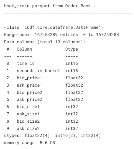
Exhibit-1: Description of book_[train/test].parquet (Image by Author)

This file is 5.6 GB and contains more than 167 million entries. There are 112 stocks and 3830 10-minute time windows (time_id). Each time window (bucket) has a maximum of 600 seconds. As one transaction intention can occur per second in each time window for each stock, the multiplication of the mentioned numbers can explain why we have millions of entries. A caveat is that not every second a transaction intention occurs, meaning that some seconds in a particular time window are missing.

  1. trade_[train/test].parquet: A parquet file, which is partitioned by stock_id, contains data on trades that are actually executed.

Feature columns in trade_[train/test].parquet:

  • stock_id — Same as above.
  • time_id — Same as above.
  • seconds_in_bucket — Same as above. Note that since trade and book data are taken from the same time window and trade data is more sparse in general, this field is not necessarily starting from 0.
  • price — The average price of executed transactions happening in one second. Prices have been normalized and the average has been weighted by the number of shares traded in each transaction.
  • size — The total number of shares traded.
  • order_count — The number of unique trade orders taking place.
Using RAPIDS cuDF to Leverage GPU in Feature Engineering
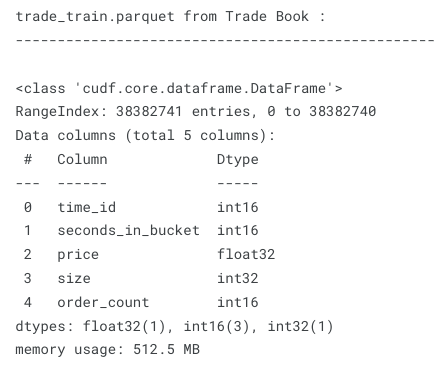
Exhibit-2: Description of trade_[train/test].parquet (Image by Author)

The trade_[train/test].parquet file is much less than book_[train/test].parquet. The former is 512.5 MB and has more than 38 million entries. Since actual transactions don’t have to match intentions, trade data is more sparse and hence fewer entries.

The goal is to predict the realized stock price volatility computed over the next 10-minute window from the feature data under the same stock_id/time_id. This project involves a great deal of feature engineering that should be performed on a large dataset. Developing new features will also increase the size of the data and the computational complexity. One remedy is to use cuDF instead of the Pandas library.

In this blog, we will see a few feature engineering tasks and data frame manipulations trying both Pandas and cuDF to compare their performances. However, we won’t use all the data but only a single stock’s records to see an exemplary implementation. One may check out the notebook to see all feature engineering work done on the entire data.

Since we execute the code on Google Colab, we should first configure our notebook to integrate Kaggle and RAPIDS.

Configuration of Google Colab Notebook

There are a few steps to configure the Colab notebook:

  1. Create an API token on the Kaggle account to authenticate the notebook with Kaggle services.

Using RAPIDS cuDF to Leverage GPU in Feature Engineering
Exhibit-3: Creating An API Token On The Kaggle Account (Image by Author)

Go to Settings and click on “Create New Token.” A file named “kaggle.json” will be downloaded which contains the username and the API key.

  1. Start a new notebook on Google Colab and upload the kaggle.json file.
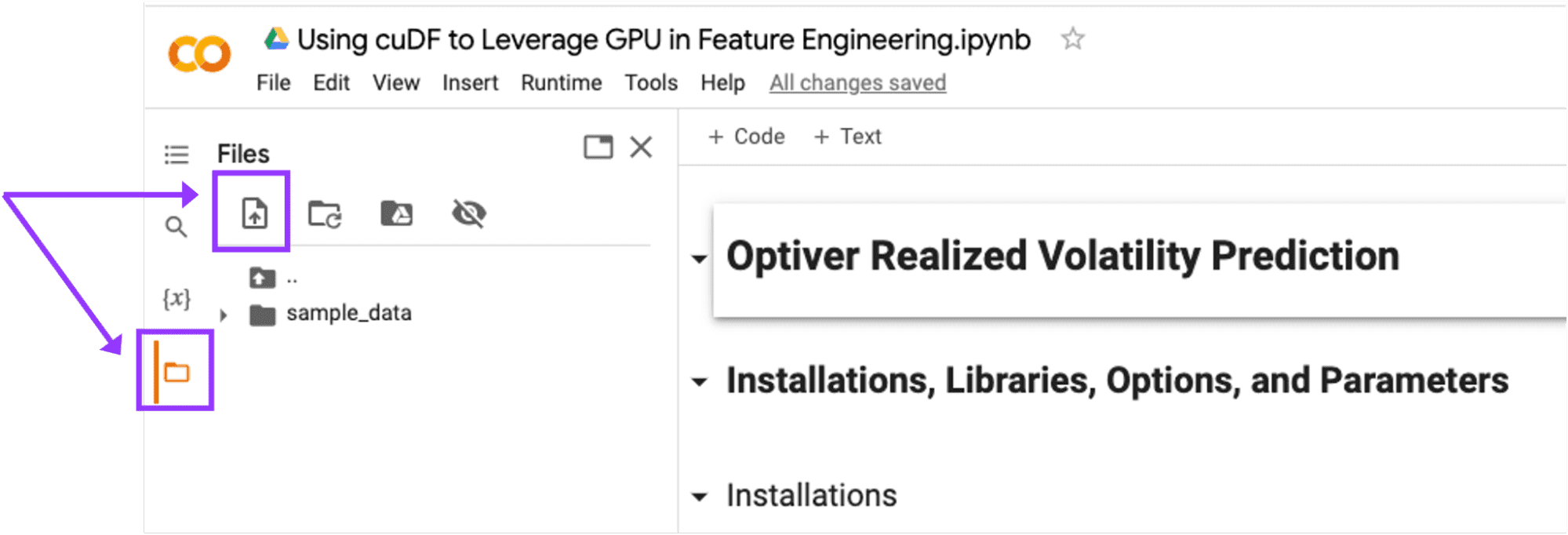
Using RAPIDS cuDF to Leverage GPU in Feature Engineering
Exhibit-4: Uploading The kaggle.json File In Google Colab (Image by Author)

Upload the kaggle.json file in Google Colab by clicking on the “Upload to session storage” icon.

  1. Click the “Runtime” dropdown at the top of the page, then “Change Runtime Type” and confirm the instance type is GPU.
  2. Execute the below command and check the output to ensure you have been allocated a Tesla T4, P4, or P100.
!nvidia-smi
  1. Get RAPIDS-Colab install-files and check your GPU:
!git clone https://github.com/rapidsai/rapidsai-csp-utils.git  !python rapidsai-csp-utils/colab/pip-install.py

Ensure that your Colab Instance is RAPIDS compatible in the output of this cell.
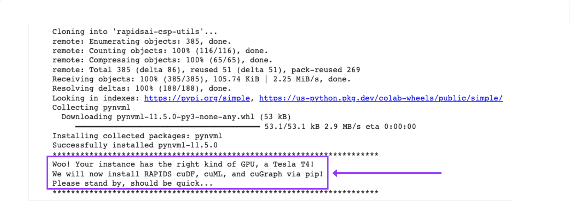
Using RAPIDS cuDF to Leverage GPU in Feature Engineering
Exhibit-5: Checking If The Colab Instance Is RAPIDS Compatible (Image by Author)

  1. Check if RAPIDS libraries are installed correctly:
import cudf, cuml  cudf.__version__

We are all set with the Google Colab configuration if the setup renders no error. Now, we can upload the Kaggle dataset.

Importing and Uploading the Kaggle Dataset

We need to make a few arrangements in our Colab instance to import the dataset from Kaggle.

  1. Install the Kaggle library:
!pip install -q kaggle
  1. Make a directory named “.kaggle”:
!mkdir ~/.kaggle
  1. Copy the “kaggle.json” into this new directory:
!cp kaggle.json ~/.kaggle/
  1. Allocate the required permission for this file:
!chmod 600 ~/.kaggle/kaggle.json
  1. Download the dataset from Kaggle:
!kaggle competitions download optiver-realized-volatility-prediction
  1. Create a directory for unzipped data:
!mkdir train
  1. Unzip data in the new directory:
!unzip optiver-realized-volatility-prediction.zip -d train
  1. Import all other libraries we need:
import glob  import numpy as np  import pandas as pd  from cudf import DataFrame  import matplotlib.pyplot as plt  from matplotlib import style  from collections import defaultdict  from IPython.display import display  import gc  import time  import warnings  %matplotlib inline
  1. Set Pandas options:
pd.set_option("display.max_colwidth", None)  pd.set_option("display.max_columns", None)  warnings.filterwarnings("ignore")    print("Threshold:", gc.get_threshold())  print("Count:", gc.get_count())
  1. Define parameters:
# Data directory that contains files  DIR = "/content/train/"    # Number of execution cycles  ROUNDS = 30
  1. Get files:
# Get order and trade books  order_files = glob.glob(DIR + "book_train.parquet" + "/*")  trade_files = glob.glob(DIR + "trade_train.parquet" + "/*")  print(order_files[:5])  print("n")  print(trade_files[:5])  print("n")    # Get stock_ids as a list  stock_ids = sorted([int(file.split('=')[1]) for file in order_files])  print(f"{len(stock_ids)} stocks: n {stock_ids} n")

Now, our notebook is ready to run all data frame tasks and perform feature engineering.

Feature Engineering

This section will discuss 13 typical engineering operations on Pandas data frame and cuDF. We will see how long these operations take and how much memory they use. Let us start by loading the data first.

1. Loading data

def load_dataframe(files, dframe=0):       print("LOADING DATA FRAMES", "n")         # Load the pandas dataframe     if dframe == 0:       print("Loading pandas dataframe..", "n")       start = time.time()       df_pandas = pd.read_parquet(files[0])       end = time.time()       elapsed_time = round(end-start, 3)       print(f"For pandas dataframe: n start time: {start} n end time: {end} n elapsed time: {elapsed_time} n")       return df_pandas, elapsed_time       # Load the cuDF dataframe     else:       print("Loading cuDF dataframe..", "n")       start = time.time()       df_cudf = cudf.read_parquet(files[0])       end = time.time()       elapsed_time = round(end-start, 3)       print(f"For cuDF dataframe: n start time: {start} n end time: {end} n elapsed time: {elapsed_time} n ")         return df_cudf, elapsed_time

When dframe=0, data will be loaded as a Pandas data frame, otherwise cuDF. For example,

Pandas:

# Load pandas order dataframe and calculate time  df_pd_order, _ = load_dataframe(order_files, dframe=0)  display(df_pd_order.head())

This will return the first five records of the Order Book (book_[train/test].parquet):
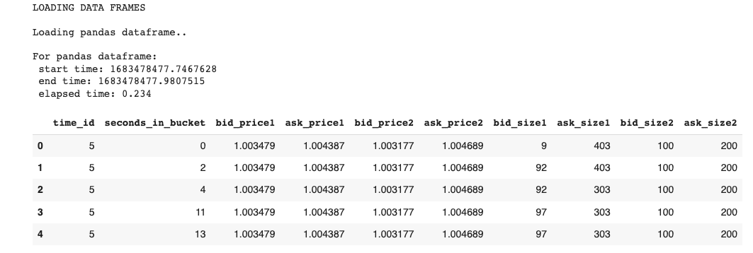
Using RAPIDS cuDF to Leverage GPU in Feature Engineering
Exhibit-6: Loading The Data As Pandas Dataframe (Image by Author)

cuDF:

# Load cuDF book dataframe and calculate time  df_cudf_order, _ = load_dataframe(order_files, dframe=1)  display(df_cudf_order.head())

Output:
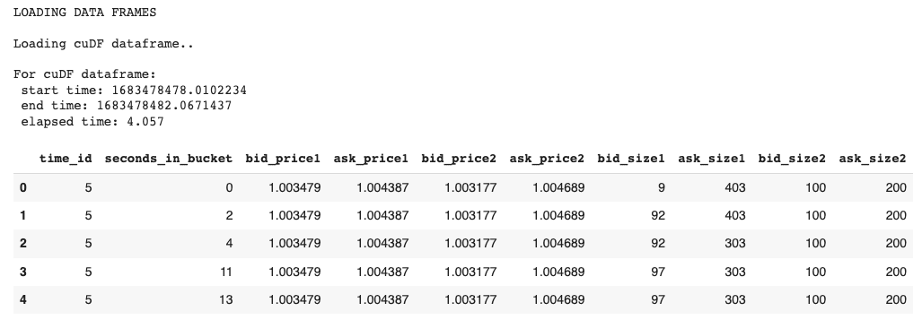
Using RAPIDS cuDF to Leverage GPU in Feature Engineering
Exhibit-7: Loading The Data As cuDF (Image by Author)

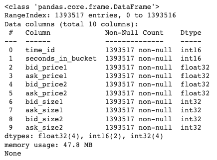
Let us get information about the Order Book data from the Pandas version:

# Order dataframe info  display(df_pd_order.info())

Output:
Using RAPIDS cuDF to Leverage GPU in Feature Engineering
Exhibit-8: Information About The First Stock’s Order Book Data (Image by Author)

The above image tells us that the first stock has around 1.4 million entries and holds 47.8 MB of memory space. To reduce the space and increase the speed, we should convert data types to lesser formats, which we’ll do later.

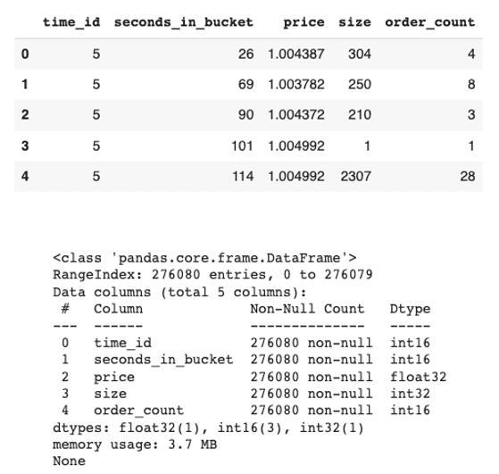
In a similar fashion, we load the Trade Book (trade_[train/test].parquet) data in both data frame libraries as we did for the Order Book data. The data and its information will look like this:
Using RAPIDS cuDF to Leverage GPU in Feature Engineering
Exhibit-9: The First Stock’s Trade Book Data And Data Info (Image by Author)

The trading data for the first stock is 3.7 MB and has over 276 thousand records.

In both files (Order Book and Trade Book), not every time window has 600 points of seconds. In other words, a particular time bucket may have transactions or bids only on some seconds in the 10-minute interval. That makes us face sparse data in both files where some seconds are missing. We should fix it by forward-filling all columns for the missing seconds. While Pandas allows us to forward fill, cuDF doesn’t have that feature. Thus, we will do forward-filling in Pandas and re-create the cuDF from the forward-filled Pandas data frame. We feel remorse about this as the central goal of this blog is to show how cuDF outperforms Pandas. I checked into the matter multiple times in the past, but to the best knowledge, I couldn’t come across the method in cuDF as implemented in Pandas. Thus, we can do forward-filling as follows[4]:

# Forward fill data  def ffill(df, df_name="order"):         # Forward fill     df_pandas = df.set_index(['time_id', 'seconds_in_bucket'])       if df_name == "order":       df_pandas = df_pandas.reindex(pd.MultiIndex.from_product([df_pandas.index.levels[0], np.arange(0,600)], names = ['time_id', 'seconds_in_bucket']), method='ffill')       df_pandas = df_pandas.reset_index()           else:       df_pandas = df_pandas.reindex(pd.MultiIndex.from_product([df_pandas.index.levels[0], np.arange(0,600)], names = ['time_id', 'seconds_in_bucket']))       # Fill nan values with 0       df_pandas = df_pandas.fillna(0)       df_pandas = df_pandas.reset_index()          # Convert to a cudf dataframe     df_cudf = cudf.DataFrame.from_pandas(df_pandas)       return df_pandas, df_cudf  

Let’s take the order data as an example and how it is processed:

# Forward fill order dataframes  expanded_df_pd_order, expanded_df_cudf_order = ffill(df_pd_order, df_name="order")  display(expanded_df_cudf_order.head())

Using RAPIDS cuDF to Leverage GPU in Feature Engineering
Exhibit-10: Forward Filling The Order Data (Image by Author)

Unlike the data in Exhibit 7, the forward-filled data in Exhibit 10 has all 600 seconds in the time bucket “5” as from 0 to 599, inclusive. We do the same operation on the trade data as well.

2. Merging Data Frames

We have two datasets, order and trade, and both are forward-filled. Both datasets are represented in Pandas and cuDF frameworks. Next, we will merge order and trade datasets on time_id and seconds_in_buckets.

def merge_dataframes(df1, df2, dframe=0):       print("MERGING DATA FRAMES", "n")         if dframe == 0:       df_type = "Pandas"     else:       df_type = "cuDF"       # Merge dataframes     print(f"Merging {df_type} dataframes..", "n")     start = time.time()     df = df1.merge(df2, how="left", on=["time_id", "seconds_in_bucket"], sort=True)     end = time.time()     elapsed_time = round(end-start, 3)     print(f"For {df_type} dataframes: n start time: {start} n end time: {end} n elapsed time: {elapsed_time} n")       return df, elapsed_time

cuDF will execute the following command:

# Merge cuDF order and trade dataframes  df_cudf, cudf_merge_time = merge_dataframes(expanded_df_cudf_order, expanded_df_cudf_trade, dframe=1)  display(df_cudf.head())

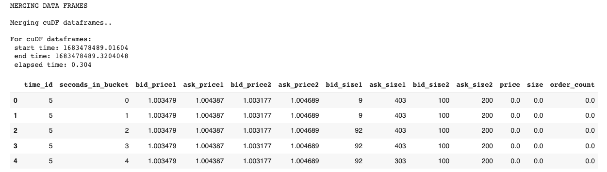
expanded_df_cudf_trade is the forward-filled trade data and is obtained the same way as expanded_df_pd_order or expanded_df_cudf_order. Merge operation will create a combined data frame as shown below:
Using RAPIDS cuDF to Leverage GPU in Feature Engineering
Exhibit-11: Merging Data Frames (Image by Author)

All columns of the two datasets are combined into one. Merging operation is repeated for the Pandas data frames too.

Using RAPIDS cuDF to Leverage GPU in Feature Engineering

3. Changing Dtype

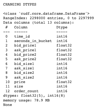
We want to change the data type of some columns to reduce memory space and increase computation speed.

# Make dtype changes  def change_dtype(df, dframe=0):       print("CHANGING DTYPES", "n")       convert_dict = {"time_id": "int16",                     "seconds_in_bucket": "int16",                     "bid_size1": "int16",                     "ask_size1": "int16",                     "bid_size2": "int16",                     "ask_size2": "int16",                     "size": "int16",                     "order_count": "int16"                     }        df = df.astype(convert_dict)       return df, dframe

When we execute the below command,

# Make dtype changes for cuDF data frame  df_cudf, _ = change_dtype(df_cudf)  display(df_cudf.info())

we get the following output:
Using RAPIDS cuDF to Leverage GPU in Feature Engineering
Exhibit-12: Changing Dtype (Image by Author)

The data in Exhibit 12 would use more memory space if no data type conversion took place. It still has 78.9 MB but, that was after the forward-fill and merge operations, which resulted in 13 columns and 2.3 million entries.

We fulfill every feature engineering task for both Pandas DF and cuDF. Here, we just showed the one for cuDF as an example.

4. Getting Unique Time Ids

We will use the unique method to extract the time_ids in this section.

# Get unique values in time_id column and put them in a list  def get_unique_timeids(df, dframe=0):       global time_ids       print("GETTING UNIQUE VALUES", "n")       # Get unique time_ids     if dframe == 0:       print(f"Getting sorted unique time_ids from Pandas dataframe..", "n")       start = time.time()       time_ids = sorted(df['time_id'].unique().tolist())       end = time.time()       elapsed_time = round(end-start, 3)       print(f"Unique time_ids from Pandas dataframe: n start time: {start} n end time: {end} n elapsed time: {elapsed_time} n")       else:       print(f"Getting sorted unique time_ids from cuDF dataframe..", "n")       start = time.time()       time_ids = sorted(df['time_id'].unique().to_arrow().to_pylist())       end = time.time()       elapsed_time = round(end-start, 3)       print(f"Unique time_ids from cuDF dataframe: n start time: {start} n end time: {end} n elapsed time: {elapsed_time} n")       print(f"{len(time_ids)} time buckets: n {time_ids[:10]}...")     print("n")       return df, time_ids

The above code will get the unique time_ids from Pandas DF and cuDF.

# Get time_ids from cuDF dataframe  time_ids = get_unique_timeids(df_cudf_order, dframe=1)

The output of the cuDF looks like this:
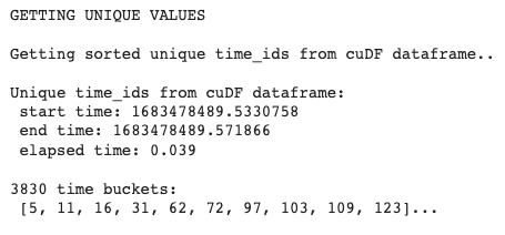
Using RAPIDS cuDF to Leverage GPU in Feature Engineering
Exhibit-13: Getting Unique Time Ids (Image by Author)

5. Checking Null Values

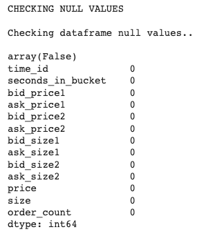
Then, we will check the null values in data frames.

# Check df null values  def check_null_values(df, dframe=0):       print("CHECKING NULL VALUES", "n")       print("Checking dataframe null values..", "n")     display(df.isna().values.any())     display(df.isnull().sum())       return df, dframe

Checking null values example in cuDF:

# Check null values for cuDF dataframe  df_cudf, _ = check_null_values(df_cudf, dframe=0)

And the output is:
Using RAPIDS cuDF to Leverage GPU in Feature Engineering
Exhibit-14: Checking Null Values (Image by Author)

6. Adding a Column

We want to create more features, so add a few columns.

# Add columns  def add_column(df, dframe=0):       print("ADDING COLUMNS", "n")       # Calculate WAPs     df['wap1'] = (df['bid_price1'] * df['ask_size1'] + df['ask_price1'] * df['bid_size1']) / (df['bid_size1'] + df['ask_size1'])     df['wap2'] = (df['bid_price2'] * df['ask_size2'] + df['ask_price2'] * df['bid_size2']) / (df['bid_size2'] + df['ask_size2'])       # Calculate order volumes     df['bid1_volume'] = df['bid_price1'] * df['bid_size1']     df['bid2_volume'] = df['bid_price2'] * df['bid_size2']     df['ask1_volume'] = df['ask_price1'] * df['ask_size1']     df['ask2_volume'] = df['ask_price2'] * df['ask_size2']       # Calculate volume imbalance     df['imbalance'] = np.absolute((df['ask_size1'] + df['ask_size2']) - (df['bid_size1'] + df['bid_size2']))       # Calculate trade volume imbalance     df['volume_imbalance'] = np.absolute((df['bid_price1'] * df['bid_size1']) - (df['ask_price1'] * df['ask_size1']))       return df, dframe

That will create new features such as weighted average price (wap1 and wap2), order volume, and volume imbalance. In total, eight columns will be added to the data frames by executing the following:

# Add a column in cuDF dataframe  df_cudf, _ = add_column(df_cudf)  display(df_cudf.head())

It will hence give us:

Using RAPIDS cuDF to Leverage GPU in Feature Engineering
Exhibit-15: Adding Columns And Features (Image by Author)

7. Dropping a Column

We decide to get rid of two features, wap1 and wap2, by dropping their columns:

# Drop columns  def drop_column(df, dframe=0):       print("DROPPING COLUMNS", "n")       df.drop(columns=['wap1', 'wap2'], inplace=True)       return df, dframe

Implementation of dropping columns is:

# Add a column in cuDF dataframe  df_cudf, _ = drop_column(df_cudf)  display(df_cudf.head())

That leaves us with the data frames that wap1, and wap2 columns are gone!

8. Calculating Statistics by Group

Next, we calculate the mean, median, maximum, minimum, standard deviation, and the sum of some features by time_id. For this, we will use groupby and agg methods.

# Calculate statistics by selected features  def calc_agg_stats(df, dframe=0):       print("CALCULATING STATISTICS", "n")       # Statistical calculations to be made      operations = ["mean", "median", "max", "min", "std", "sum"]       # Features for which statistical calculations will be made     features_list = ["bid1_volume", "bid2_volume", "ask1_volume", "ask2_volume"]       # Create a dictionary to store feature-calculation pairs     stats_dict = defaultdict(list)     for feature in features_list:         stats_dict[feature].extend(operations)       # Calculate aggregate statistics     df_stats = df.groupby('time_id', as_index=False, sort=True).agg(stats_dict)       return df, df_stats

We create a list named features_list to specify the features that the mathematical calculations will be performed.

# Calculate statistics by selected features in cuDF dataframe  _, df_cudf_stats = calc_agg_stats(df_cudf)  display(df_cudf_stats.head())

In return, we get the following output:

Using RAPIDS cuDF to Leverage GPU in Feature Engineering
Exhibit-16: Calculating Statistics (Image by Author)

The returned table is a new data frame. We should merge it with the original one (df_cudf). We will accomplish it through Pandas:

# Merge data frame with stats  def merge_dataframes_2(df, dframe=0):       if dframe == 0:       df = df.merge(df_pd_stats, how="left", on="time_id", sort=True)         else:       df = df.to_pandas()       df = df.merge(df_pd_stats, how="left", on="time_id", sort=True)       df = cudf.DataFrame.from_pandas(df)       return df, dframe      # Merge cuDF data frames  df_cudf, _ = merge_dataframes_2(df_cudf, dframe=1)  display(df_cudf.head())

The above snippet will put df_pd_stats and df_pd in one data frame and save it as df_cudf.

As usual, we repeat the same task for Pandas.

The next step is to calculate the correlation between two columns:

# Calculate correlation between two selected features  def calc_corr(df, dframe=0):     correlation = df[["bid1_volume", "ask1_volume"]].corr()   print(f"Correlation between 'bid1_volume' and 'ask1_volume' is {correlation} n")     return df, correlation

This code

# Calculate correlation in cuDF dataframe  _ = calc_corr(df_cudf)

will return the following output:

Using RAPIDS cuDF to Leverage GPU in Feature Engineering
Exhibit-17: Calculating Correlation Between Two Features (Image by Author)

9. Renaming Columns

To remove any confusion, we should rename two of our columns.

# Rename columns  def rename_cols(df, dframe=0):       print("RENAMING COLUMNS", "n")       df = df.rename(columns={"imbalance": "volume_imbalance", "volume_imbalance": "trade_volume_imbalance"})       return df, dframe

Columns imbalance and volume_imbalance will be renamed as volume_imbalance and trade_volume_imbalance, respectively.

10. Binning a Column

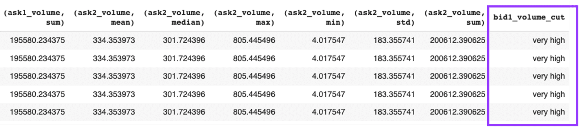
Another data manipulation we want to make is to bin the bid1_volume and store the bins in a new column.

# Bin a selected column  def bin_col(df, dframe=0):       print("BINNING A COLUMN", "n")       if dframe == 0:       df['bid1_volume_cut'] = pd.cut(df["bid1_volume"], bins=5, labels=["very high", "high", "average", "low", "very low"], ordered=True)       else:       df['bid1_volume_cut'] = cudf.cut(df["bid1_volume"], bins=5, labels=["very high", "high", "average", "low", "very low"], ordered=True)       return df, dframe

By running the lines

# Bin a selected column in cuDF dataframe  df_cudf, _ = bin_col(df_cudf, dframe=1)  display(df_cudf.head())

we’ll get a data frame as the output, which we may see a part of it as shown below:
Using RAPIDS cuDF to Leverage GPU in Feature Engineering
Exhibit-18: Binning A Column (Image by Author)

11. Displaying Data Frames

After feature engineering steps are completed, we can present the data frames. This section contains three operations: displaying the data frame, getting information about it, and describing it.

# Display data frame  def display_df(df, dframe=0):       print("DISPLAYING DATA FRAMES", "n")       display(df.head())     print("n")       return df, dframe      # Display dataframe info  def display_info(df, dframe=0):       print("DISPLAYING DATA FRAME INFO", "n")       display(df.info())     print("n")       return df, dframe      # Display dataframe info  def describe_df(df, dframe=0):       print("DESCRIBING DATA FRAMES", "n")       display(df.describe())     print("n")       return df, dframe

The following code will finalize these three tasks:

# Display cuDF dataframe and info  _, _ = display_df(df_cudf, dframe=1)  _, _ = display_info(df_cudf, dframe=1)  _, _ = describe_df(df_cudf, dframe=1)

We are done with feature engineering.

Single-Run Execution

In summary, our feature engineering efforts have focused on the following tasks:

  1. Loading data frames
  2. Merging data frames
  3. Changing data type
  4. Getting unique time_ids.
  5. Checking null values
  6. Adding columns
  7. Dropping columns
  8. Calculating statistics
  9. Calculating a correlation
  10. Renaming columns
  11. Binning a column
  12. Displaying data frames
  13. Displaying data information
  14. Describing data frames

It was all 13 tasks, but we mentioned “Calculating a correlation” as a separate entity here. Now, we want to run these tasks sequentially in a single run, as shown below:

def run_and_report():       # Create a dictionary to store elapsed times     time_dict = defaultdict(list)       # List operations to be performed     labels = ["changing_dtype",               "getting_unique_timeids",               "checking_null_values",               "adding_column",               "dropping_column",               "calculating_agg_stats",               "merging_dataframes",               "renaming_columns",               "binning_col",               "calculating_corr",               "displaying_dfs",               "displaying_info",               "describing_dfs"]       # Load pandas order dataframe and calculate time     df_pd_order, pd_order_loading_time = load_dataframe(order_files, dframe=0)     print("-"*150, "n")       # Load cuDF book dataframe and calculate time     df_cudf_order, cudf_order_loading_time = load_dataframe(order_files, dframe=1)     print("-"*150, "n")       # Load pandas trade dataframe and calculate time     df_pd_trade, pd_trade_loading_time = load_dataframe(trade_files, dframe=0)     print("-"*150, "n")       # Load cuDF trade dataframe and calculate time     df_cudf_trade, cudf_trade_loading_time = load_dataframe(trade_files, dframe=1)     print("-"*150, "n")       # Get time_ids from Pandas data frame     _, time_ids = get_unique_timeids(df_pd_order, dframe=0)     print("-"*150, "n")       # Get time_ids from cuDF dataframe     _, time_ids = get_unique_timeids(df_cudf_order, dframe=1)     print("-"*150, "n")       # Store loading times     time_dict["loading_dfs"].extend([pd_order_loading_time, cudf_order_loading_time])       # Forward fill order dataframes     expanded_df_pd_order, expanded_df_cudf_order = ffill(df_pd_order, df_name="order")       # Forward fill trade dataframes     expanded_df_pd_trade, expanded_df_cudf_trade = ffill(df_pd_trade, df_name="trade")       # Merge pandas order and trade dataframes     df_pd, pd_merge_time = merge_dataframes(expanded_df_pd_order, expanded_df_pd_trade, dframe=0)     print("-"*150, "n")       # Merge pandas order and trade dataframes     df_cudf, cudf_merge_time = merge_dataframes(expanded_df_cudf_order, expanded_df_cudf_trade, dframe=1)     print("-"*150, "n")       # Store merge times     time_dict["merging_dfs"].extend([pd_merge_time, cudf_merge_time])       # Apply functions     functions = [change_dtype,                  get_unique_timeids,                  check_null_values,                  add_column,                  drop_column,                  calc_agg_stats,                  merge_dataframes_2,                  rename_cols,                  bin_col,                  calc_corr,                  display_df,                  display_info,                  describe_df]       for label, function in enumerate(functions):         # Function for pandas       start_pd = time.time()       df_pd, x = function(df_pd, dframe=0)       end_pd = time.time()       elapsed_time_for_pd = round(end_pd-start_pd, 3)       print(f"For pandas dataframe: n start time: {start_pd} n end time: {end_pd} n elapsed time: {elapsed_time_for_pd} n")              # Function for cuDF       start_cudf = time.time()       df_cudf, x = function(df_cudf, dframe=1)       end_cudf = time.time()       elapsed_time_for_cudf = round(end_cudf-start_cudf, 3)       print(f"For cuDF dataframe: n start time: {start_cudf} n end time: {end_cudf} n elapsed time: {elapsed_time_for_cudf} n")       print("-"*150, "n")         # Store elapsed times       time_dict[labels[label]].extend([elapsed_time_for_pd, elapsed_time_for_cudf])       # Delete the unsolicited time duration     del time_dict["merging_dataframes"]     labels.remove("merging_dataframes")     labels.insert(0, "merging_dfs")     labels.insert(0, "loading_dfs")       print(time_dict)       return time_dict, labels, df_pd, df_cudf

The run_and_report function will give the same outputs as before but in a full report by a single execution command. It will execute the 14 tasks on both Pandas and cuDF and record the times they take for both data frames.

time_dict, labels, df_pd, df_cudf = run_and_report()

We may have to run multiple cycles to see the relative performance of both data libraries more boldly.

Final Evaluation

If we run the run_and_report multiple times, such as in rounds, we can get a better sense of the difference in performance between Pandas and cuDF. So, we set rounds as 30. Then, we record all time durations for every operation, round, and data library and finally evaluate the results:

def calc_exec_times():       exec_times_by_round = {}       # Calculate execution times of operations in each round     for round_no in range(1, ROUNDS+1):       # cycle_no += 1       time_dict, labels, df_pd, df_cudf = run_and_report()       exec_times_by_round[round_no] = time_dict       print("exec_times_by_round: ", exec_times_by_round)       # Get durations by operation for each data frame     pd_summary, cudf_summary = get_statistics(exec_times_by_round, labels)       # Get durations by rounds for each data frame     round_total = get_total(exec_times_by_round)     print("n"*3)       # Plot durations     plt.style.use('dark_background')     X_axis = np.arange(len(labels))       # Plot average duration of operation     plot_avg_by_df(pd_summary, cudf_summary, labels, X_axis)     print("n"*3)       # Plot total and difference in duration by operation     plot_diff_by_df(pd_summary, cudf_summary, labels)     print("n"*3)       # Plot total and difference in duration by round     plot_total_by_df(round_total)     print("n"*3)

The calc_exec_times function executes a few tasks. It first calls get_statistics to get the “average and total time durations by operation” for each data library over 30 rounds.

def get_statistics(exec_times_by_round, labels):       # Separate and store duration statistics by data frame     pd_performance = defaultdict(list)     cudf_performance = defaultdict(list)       # Get and store durations for each operation by data frame     for label in labels:       for key, values in exec_times_by_round.items():           pd_performance[label].append(values[label][0])         cudf_performance[label].append(values[label][1])       print("pd_performance: ", pd_performance)     print("cudf_performance: ", cudf_performance)       # Compute average and total durations for each operation by data frame     pd_summary = {key: [round(sum(value), 3), round(np.average(value), 3)] for key, value in pd_performance.items()}     cudf_summary = {key: [round(sum(value), 3), round(np.average(value), 3)] for key, value in cudf_performance.items()}       print("pd_summary: ", pd_summary)     print("cudf_summary: ", cudf_summary)        return pd_summary, cudf_summary

Next, it computes the “total duration by round” for each data framework.

def get_total(exec_times_by_round):       def get_round_total(stat_list):         # Get total duration by round for each data frame       pd_round_total = round(sum([x[0] for x in stat_list]), 3)       cudf_round_total = round(sum([x[1] for x in stat_list]), 3)         return pd_round_total, cudf_round_total       # Collect total durations by round     for key, value in exec_times_by_round.items():       round_total = {key: get_round_total(list(value.values())) for key, value in exec_times_by_round.items()}       print("round_total", round_total)       return round_total

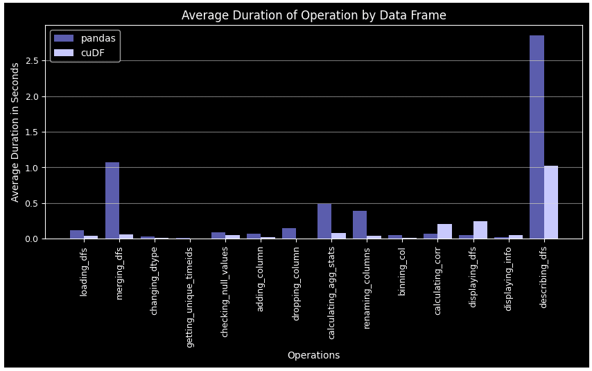
Lastly, it plots the results. Here, the first plot is for the “average time duration by operation” for both libraries.

def plot_avg_by_df(pd_summary, cudf_summary, labels, X_axis):       # Figure size     fig = plt.subplots(figsize =(10, 4))       # Average duration by operation for each data frame     pd_avg = [value[1] for key, value in pd_summary.items()]     cudf_avg = [value[1] for key, value in cudf_summary.items()]       plt.bar(X_axis - 0.2, pd_avg, 0.4, color = '#5A5AAF', label = 'pandas', align='center')     plt.bar(X_axis + 0.2, cudf_avg, 0.4, color = '#C8C8FF', label = 'cuDF', align='center')       plt.xticks(X_axis, labels, fontsize=9, rotation=90)     plt.yticks(fontsize=9)     plt.xlabel("Operations", fontsize=10)     plt.ylabel("Average Duration in Seconds", fontsize=10)     plt.grid(axis='y', color="#E4E4E4", alpha=0.5)     plt.title("Average Duration of Operation by Data Frame", fontsize=12)     plt.legend()     plt.show()
Using RAPIDS cuDF to Leverage GPU in Feature Engineering
Exhibit-19: Average Duration By Operation For Pandas Data Frame And cuDF (Image by Author)

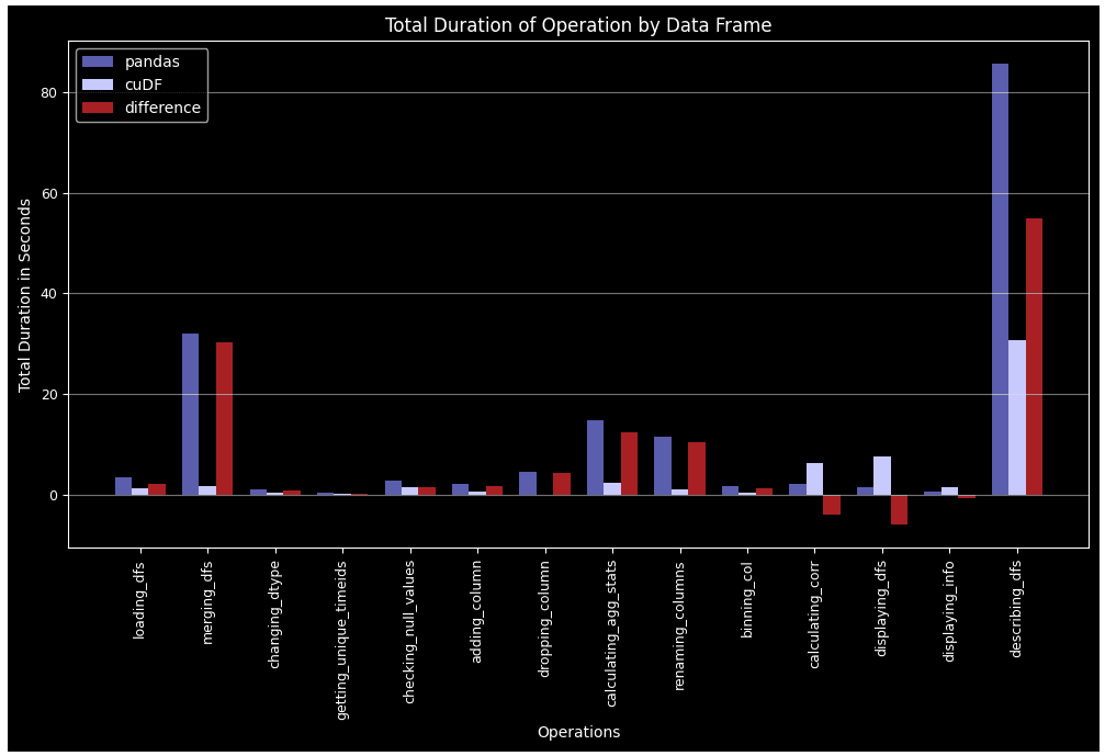
The second plot is for the “total duration by operation,” which shows the total time each task took over all 30 rounds.

def plot_diff_by_df(pd_summary, cudf_summary, labels):       # Figure size     fig = plt.subplots(figsize =(12, 6))       # Total duration by operation for each data frame     pd_total = [value[0] for key, value in pd_summary.items()]     cudf_total = [value[0] for key, value in cudf_summary.items()]       # Difference of total duration by operation for each data frame     diff = [x[0]-x[1] for x in zip(pd_total, cudf_total)]       # Set width of bar     barWidth = 0.25       # Set position of bar on X axis     br1 = np.arange(len(labels))     br2 = [x + barWidth for x in br1]     br3 = [x + barWidth for x in br2]       plt.bar(br1, pd_total, barWidth, color = '#5A5AAF', label = 'pandas', align='center')     plt.bar(br2, cudf_total, barWidth, color = '#C8C8FF', label = 'cuDF', align='center')     plt.bar(br3, diff, barWidth, color = '#AA1E1E', label = 'difference', align='center')       plt.xticks([r + barWidth for r in range(len(labels))], labels, fontsize=9, rotation=90)     plt.yticks(fontsize=9)     plt.xlabel("Operations", fontsize=10)     plt.ylabel("Total Duration in Seconds", fontsize=10)     plt.grid(axis='y', color="#E4E4E4", alpha=0.5)     plt.title("Total Duration of Operation by Data Frame", fontsize=12)     plt.legend()     plt.show()
Using RAPIDS cuDF to Leverage GPU in Feature Engineering
Exhibit-20: Total Duration By Operation Over 30 Rounds For Pandas Data Frame And cuDF (Image by Author)

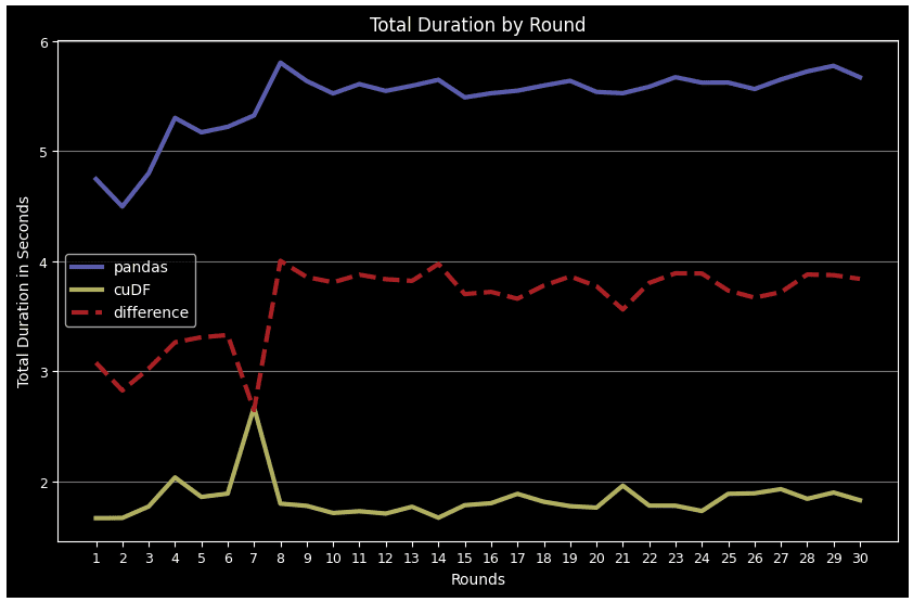
The final plot is “total duration by round,” which shows the total time all operations took together for each round.

def plot_total_by_df(round_total):        # Figure size     fig = plt.subplots(figsize =(10, 6))       X_axis = np.arange(1, ROUNDS+1)       # Total duration by round for each data frame     pd_round_total = [value[0] for key, value in round_total.items()]     cudf_round_total = [value[1] for key, value in round_total.items()]       # Difference of total duration by round for each data frame     diff = [x[0]-x[1] for x in zip(pd_round_total, cudf_round_total)]       plt.plot(X_axis, pd_round_total, linestyle="-", linewidth=3, color = '#5A5AAF', label = "pandas")     plt.plot(X_axis, cudf_round_total, linestyle="-", linewidth=3, color = '#B0B05A', label = "cuDF")     plt.plot(X_axis, diff, linestyle="--", linewidth=3, color = '#AA1E1E', label = "difference")       plt.xticks(X_axis, fontsize=9)     plt.yticks(fontsize=9)     plt.xlabel("Rounds", fontsize=10)     plt.ylabel("Total Duration in Seconds", fontsize=10)     plt.grid(axis='y', color="#E4E4E4", alpha=0.5)     plt.title("Total Duration by Round", fontsize=12)     plt.legend()     plt.show()
Using RAPIDS cuDF to Leverage GPU in Feature Engineering
Exhibit-21: Total Duration Of All Operations For Each Round For Pandas Data Frame And cuDF (Image by Author)

Even though we haven’t covered every feature engineering task fulfilled on the dataset, they are the same as or similar to the ones we showed here. By explaining 14 operations individually, we tried to document the relative performance of Pandas data frame and cuDF, and enable reproducibility.

In all cases except for correlation calculation and data frame display, cuDF surpasses Pandas. This performance lead becomes more remarkable in complex tasks such as groupby, merge, agg, and describe. Another point is Pandas DF gets tired over time when more rounds come over, while cuDF follows a more stable pattern.

Recall that we have reviewed only one stock as an example. If we process all 112 stocks, we may expect a larger performance gap in favor of cuDF. If the stock's population goes up to the hundreds, cuDF’s performance can even be more dramatic. In the case of big data, where the execution of parallel tasks is possible, a distributed framework such as Dask-cuDF, which extends parallel computing to cuDF GPU DataFrames, can be the right tool.

References

[1] RAPIDS Definition, https://www.heavy.ai/technical-glossary/rapids

[2] 10 Minutes to cuDF and Dask-cuDF, https://docs.rapids.ai/api/cudf/stable/user_guide/10min/

[3] Optiver Realized Volatility Prediction, https://www.kaggle.com/competitions/optiver-realized-volatility-prediction/data

[4] Forward filling book data, https://www.kaggle.com/competitions/optiver-realized-volatility-prediction/discussion/251277
Hasan Serdar Altan is Data scientist and AWS Cloud Architect Associate.

More On This Topic

  • RAPIDS cuDF Cheat Sheet
  • RAPIDS cuDF to Speed up Your Next Data Science Workflow
  • RAPIDS cuDF for Accelerated Data Science on Google Colab
  • Feature Store Summit 2022: A free conference on Feature Engineering
  • Date Processing and Feature Engineering in Python
  • Feature Engineering of DateTime Variables for Data Science, Machine…

73% of consumers trust what generative AI wants us to see

Blue lines representing abstract AI

Keen to use generative artificial intelligence (AI) to save effort and time, 73% of consumers trust content produced by such tools, with those in Norway and Singapore among the most and least trusting, respectively.

At 51%, just over half were aware of the latest generative AI trends and had explored the available tools, according to a survey that polled 10,000 respondents across 13 markets, including Australia, Japan, Sweden, the US, and the UK. The findings were released by Capgemini Research Institute, which conducted the study for search analysis between April 2022 and March 2023 as well as for social analysis from October 2022 to April 2023.

Also: The best AI chatbots

About 52% use generative AI tools to generate content such as email and essays, while 28% tap the technology for brainstorming, and 23% use the tools to gather general information on a range of topics, including science, history, and technology.

Chatbots are the most popular, used by 15% of respondents who tap generative AI tools multiple times a week, followed by games such as generative AI-powered game studios or applications, which are used by 11% of respondents.

Capgemini further noted that AI art featuring anime characters was popular among respondents in Asia-Pacific and Canada, but users expressed caution about using generative AI here due to incorrect or inaccurate results.

Across the board, trust in content generated by such tools was the highest in Norway at 79%, followed by 75% in Spain. The lowest level of trust was in Singapore and Germany, at 70% in each of the markets.

Also: How to access, install, and use AI ChatGPT-4 plugins (and why you should)

Capgemini attributed the high trust level possibly to the enhanced efficiency generated by these tools as well as the availability of personalized content in a "ready-to-use format", particularly for tasks such as software coding and multimedia creation.

"Tools such as ChatGPT respond to users' prompts in a clear, easily understood manner, and it is possible consumers equate this clarity with accuracy," the report noted. "Further, popular generative AI applications such as ChatGPT are backed by renowned tech firms such as Microsoft and Alphabet, which endorsements also increase consumer trust levels."

More than half, 53% globally, said they trust generative AI to help with their financial planning. Tools in this space include Alpha, which is powered by OpenAI's GPT-4, and FinChat, also powered by ChatGPT.

Also: Is humanity really doomed? Consider AI's Achilles heel

In addition, 67% said they could benefit from receiving medical diagnoses and advice from generative AI, with another 63% excited about the possibility of generative AI supporting more accurate and efficient drug discovery. Some 66% would seek out generative AI-powered advice for personal relationships or life and career plans.

At 49%, just under half said they were not concerned about the potential for generative AI to be used to create fake news stories. Just 34% were concerned about phishing attacks, while 33% expressed concerns about copyright issues, and an even lower 27% were worried about the use of generative AI tools to copy competitor's product designs.

"The awareness of generative AI among consumers globally is remarkable and the rate of adoption has been massive. Yet, the understanding of how this technology works and the associated risks are still very low," said Niraj Parihar, CEO of Capgemini's insights and data global business line. "While regulation is critical, business and technology partners also have an important role to play in providing education and enforcing the safeguards that address concerns around the ethics and misuse of generative AI."

Also: Generative AI: Just don't call it an 'artist' says scholars in Science magazine

Noting that Capgemini helps its clients create use cases within an ethical framework, Parihar said: "Generative AI is not 'intelligent' in itself; the intelligence stems from the human experts who these tools will assist and support. The key to success, therefore, as with any AI, is the safeguards that humans build around them to guarantee the quality of its output."

The study found that 43% were keen for businesses to apply generative AI across customer interactions, with another 70% already using such tools for product or service recommendations, in place of traditional methods such as search.

What the World Can Learn From France’s AI Ecosystem

During a tech conference in Paris this week, French President Emmanuel Macron announced not just a 500 million euro ($540 million) investment, but with it an aim to ensure competitiveness of its AI ecosystem. It looks like France is bearing the fruit of its futuristic planning, policy framing and strategic alignment around the industry. This comes in the backdrop of a young AI startup—Mistral AI receiving a seed funding of a jaw-dropping $113 million.

The AI race is no longer limited to the big techs and the US and China, and is open to all the nations and the open-source community at large. France looks determined to establish itself as a technology and AI superpower. It aims to leverage its assets to foster innovation and development in AI. Even countries like Abu Dhabi and Saudi Arabia are heavily investing in AI.

While the US has been a clear leader for decades, with researchers, academics and tech companies headquartered in the US, China has also rapidly ramped up its research output and investment. Additionally, nations like the UK, Canada, and Japan have also made strides. Europe seems to be lagging behind, while Germany and France have toiled their way up.

France vs the World

France has been one of the hubs of artificial intelligence research for many years. It has a strong tradition of research in mathematics, computer science, and statistics, which has provided a foundation for AI research.

France’s AI strategy led to a number of major developments in the country’s AI ecosystem. It fostered the creation of many new AI research centres and institutes such as the 3IA institutes and the Inria Paris-Saclay Center for Artificial Intelligence. Numerous AI startups such as Criteo, Dataiku, and Owkin also came into being. Additionally, it also drew investment from large multinational companies such as Air France, Renault, and Total for research and development AI.

France also boasts of prominent AI researchers and entrepreneurs, including Meta AI chief Yann LeCun, Keras creator François Chollet, Google AI director Sylvain Gelly, Dataiku chief Nicolas Usunier, former Apple exec Luc Julia, and Hugging Face’s co-founder Clem Delangue.

In recent years, the French government has also made AI a priority, and has invested heavily in AI research and development. In 2018, the country launched a €1.5 billion national AI strategy, which aims to make France a global leader in AI. The strategy includes funding for research, education, and the development of AI applications.

Paving a way for sustainability

Another thing that France can bank upon is its reliance on nuclear power plants for about 70% of the energy used in France is generated by nuclear power plants. Years of research and funding have made nuclear power generation technology adaptable for smaller industrial applications such as data centres. This has paved the way for utilising nuclear energy to power AI data centers, which have substantial energy requirements and can contribute to environmental pollution.

This makes France a very attractive location for data centres, as it can offer a reliable and affordable source of power. Nuclear power can also helpAI data centers reduce their carbon footprint and operate in a more sustainable manner.

Open source advocate

The French President, during the event in Paris, made a speech that sparked an intriguing debate on AI. He advocated for a balanced approach to regulation that addresses potential risks without stifling innovation and competition at various levels of the AI stack. He, however, emphasised on the significance of preventing all the value and power from accumulating solely in the hands of major American AI companies and ensuring that new French companies can participate and build upon open source AI systems. Macron envisioned a future where both proprietary and open-source systems coexist, highlighting the advantages and disadvantages of each.

France has been one of the biggest contributors to the open-source ecosystem. Meta’s open-source large language model LLaMA was developed and deployed by researchers from Paris.

Not just that Hugging Face — a platform that actively engages with the open-source community and plays a significant role in fostering collaboration and knowledge sharing within the field of NLPs — has its roots in Paris as well. The firm is headquartered in New York but itsresearch team is based in Paris. Hugging Face also has a number of partnerships with French universities and research institutions.

Also the new generative AI superstar in town Mistral AI is based in Paris. The co-founders Arthus Mensch and Guillaume Lample are French nationals and have worked at DeepMind and Meta AI, respectively. Lample is one of the core members of the team behind Meta AI’s LLaMa model, which has been leading the way in open-source. The duo also emphasises an open-source approach, and are aiming to build solutions for enterprises rather than consumer-centric products. They believe that making AI useful is a major challenge and intend to release their products to the market in 2024.

LeCun is also an advocate for open source software, and co-founded PyTorch, a popular open-source deep learning library widely used by researchers, developers, and businesses worldwide. He also believes open source plays a vital role in advancing artificial intelligence.

What about India?

As the world steps into an era of hands-on AI innovation, India is still languishing in theory. “When it comes to theoretical work, we are as good as anyone… But the latest advances have gone beyond theory. The gap has further widened which we need to bridge,” Prof Amrutur Bharadwaj, research head and director, ARTPARK, told AIM.

India’s top universities like IISc rank amongst one of the lowest at 161 on Nature’s index for high quality research. India can learn from France’s futuristic vision to invest in establishing a research-oriented ecosystem focused on AI to drive growth.

The post What the World Can Learn From France’s AI Ecosystem appeared first on Analytics India Magazine.

Calculate Computational Efficiency of Deep Learning Models with FLOPs and MACs

What are FLOPs and MACs?

FLOPs (Floating Point Operations) and MACs (Multiply-Accumulate Operations) are metrics that are commonly used to calculate the computational complexity of deep learning models. They are a fast and easy way to understand the number of arithmetic operations required to perform a given computation. For example, when working with different model architectures such as MobileNet or DenseNet for edge devices, people use MACs or FLOPs to estimate the model performance. Also, the reason we use the word “estimate” is that both metrics are approximations instead of the actual capture of the runtime performance model. However, they still can provide very useful insights on energy consumption or computational requirements, which is quite useful in edge computing.

Calculate Computational Efficiency of Deep Learning Models with FLOPs and MACs
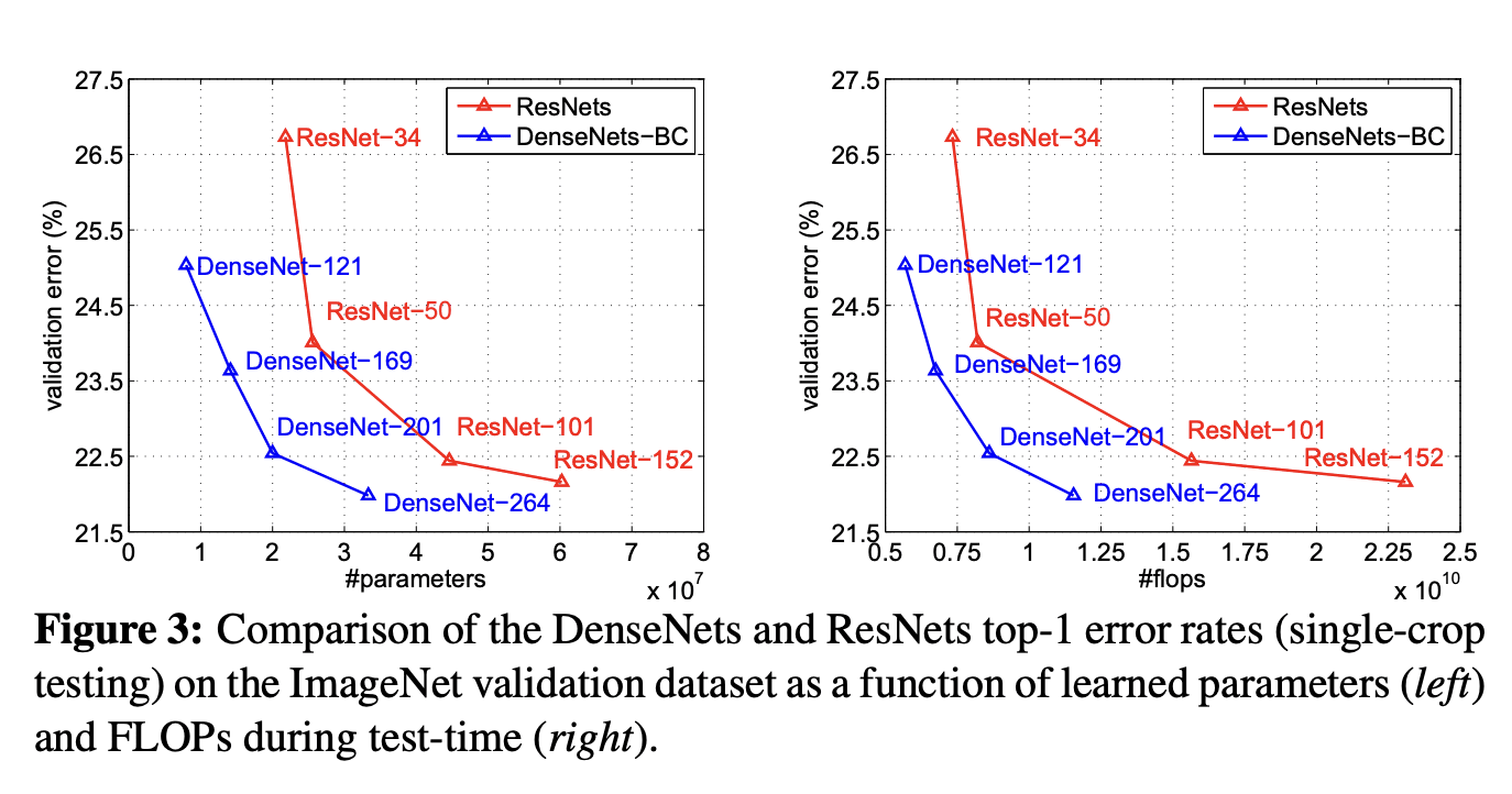
Figure 1: Comparison of different neural nets using FLOPs from “Densely Connected Convolutional Networks”

FLOPs specifically refer to the number of floating-point operations, which include addition, subtraction, multiplication, and division operations on floating-point numbers. These operations are prevalent in many mathematical computations involved in machine learning, such as matrix multiplications, activations, and gradient calculations. FLOPs are often used to measure the computational cost or complexity of a model or a specific operation within a model. This is helpful when we need to provide an estimation of the total arithmetic operations required, which is generally used in the context of measuring computation efficiency.

MACs, on the other hand, only count the number of multiply-accumulate operations, which involve multiplying two numbers and adding the result. This operation is fundamental to many linear algebra operations, such as matrix multiplications, convolutions, and dot products. MACs are often used as a more specific measure of computational complexity in models that heavily rely on linear algebra operations, such as convolutional neural networks (CNNs).

One thing worth mentioning here is that FLOPs cannot be the single factor that people calculate to get a sense of computation efficiency. Many other factors are considered necessary when estimating the model efficiency. For example, how parallel the system setup is; what architecture model has(e.g. group convolution costs in MACs); what computing platform the model uses(e.g. Cudnn has GPU acceleration for deep neural networks and standard operations such as forward or normalization are highly tuned).

Are FLOPS and FLOPs the Same?

FLOPS with all uppercase is the abbreviation of “floating point operations per second”, which refers to the computation speed and is generally used as a measurement of hardware performance. The "S" in the "FLOPS" stands for "second" and together with "P" (as "per"), it is generally used to represent a rate.

FLOPs(lowercase “s” stands for plural) on the other hand, refers to the floating-point operations. It is commonly used to calculate the computation complexity of an algorithm or model. However, in the discussion of AI, sometimes FLOPs can have both of the above meanings and it will leave it to the reader to identify the exact one it stands for. There have also been some discussions calling for people to abandon the usage of “FLOPs” completely and use “FLOP” instead so it’s easier to tell each one apart. In this article, we will continue to use FLOPs.

Relationship between FLOPs and MACs

Relationship between FLOPs and MACs
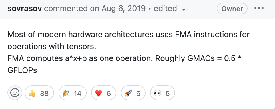
Figure 2: Relationship between GMACs and GLOPs(source)

As mentioned in the previous section, the major difference between FLOPs and MACs include what types of arithmetic operations they count and the context in which they are used. The general AI community consensus, like the GitHub comment in Figure 2, is one MACs equals roughly two FLOPs. For deep neural networks, multiply-accumulate operations are heavy in calculations therefore MACs is considered more significant.

How to Calculate FLOPs?

The good thing is there are multiple open-source packages available already for calculating FLOPs specifically so you don’t have to implement it from scratch. Some of the most popular ones include flops-counter.pytorch and pytorch-OpCounter. There are also packages such as torchstat that gives users a general network analyzer based on PyTorch. It is also worth noting that for these packages the supported layers and models are limited. So if you are running a model that consists of customized network layers you might have to calculate FLOPs yourself.

Here we show a code example to calculate FLOPs using pytorch-OpCounter and a pre-trained alexnet from torchvision:

from torchvision.models import alexnet  from thop import profile    model = alexnet()  input = torch.randn(1, 3, 224, 224)  macs, params = profile(model, inputs=(input, ))  

Conclusion

In this article, we introduced the definition of FLOPs and MACs, when they are usually used and the difference between the two attributes.

References

  • https://github.com/sovrasov/flops-counter.pytorch
  • https://github.com/Lyken17/pytorch-OpCounter
  • https://github.com/Swall0w/torchstat
  • https://arxiv.org/pdf/1704.04861.pdf
  • https://arxiv.org/abs/1608.06993

Danni Li is the current AI Resident at Meta. She's interested in building efficient AI systems and her current research focus is on-device ML models. She is also a strong believer of open source collaboration and utilizing community support to maximize our potential for innovation.

More On This Topic

  • How To Calculate Algorithm Efficiency
  • Computational Complexity of Deep Learning: Solution Approaches
  • Deep Learning Recommendation Models (DLRM): A Deep Dive
  • How to deploy Machine Learning/Deep Learning models to the web
  • How to calculate confidence intervals for performance metrics in Machine…
  • High-Performance Deep Learning: How to train smaller, faster, and better…

France’s Bid to Become Europe’s AI Hub: A Potential Challenge for the U.S

In a bold move to solidify its position on the global artificial intelligence (AI) map, France is strategically gearing up to become Europe's principal hub for AI. This development is not only set to challenge European nations but also aims to redefine the established hierarchy of global tech giants, particularly the United States. The ambitious drive to shape France as the epicenter of the expanding AI landscape was recently detailed in a CNBC report.

France's Comprehensive AI Strategy

The cornerstone of France's AI agenda is a thorough strategy involving considerable public and private sector investments. The French government has unfurled a national AI scheme, directing massive funding into AI research and development. This is not merely about pouring money into the sector, but creating a holistic environment conducive to AI innovation. It aims to strengthen both the academic and commercial sectors of AI, making France an attractive destination for AI talents and enterprises.

Interestingly, the tech industry is positively responding to France's supportive ecosystem. Giants such as Google and Facebook have already set up AI research centers in Paris. Simultaneously, several budding AI startups have chosen France as their launching pad. This synchronized effort from the public and private sectors is gradually shaping France into a nucleus of AI innovation within the European Union.

A Challenge for the U.S and a New Global AI Dynamic

France's ambition to emerge as Europe's AI hub presents a significant challenge to the U.S., the longstanding global AI leader. France's accelerated growth in the field of AI could potentially redirect talents and investments that would traditionally flow towards the U.S., creating a shift in the global AI dynamics. While this could unsettle established hierarchies, it also provides an opportunity for a more diverse and collaborative global AI ecosystem.

We are moving towards a future where the insights and breakthroughs in AI will come from a more varied set of players. The decentralization of AI dominance could lead to the flourishing of a more inclusive and cooperative international AI environment. It could pave the way for diverse AI-driven solutions and ideas, fostered by the unique cultural, economic, and social contexts of different regions.

Forecasting the Future of AI in France

Looking forward, the sustainability of France's AI strategy will largely depend on its commitment to nurturing these initiatives. The challenge lies in remaining an attractive AI hotspot that can keep pulling in talents and investments amidst the rapidly evolving global AI landscape. Considering the firm resolve shown by both the government and the private sector, France's vision to become Europe's AI hub appears increasingly plausible.

France's strategic push towards AI dominance signifies the escalating global competitiveness of this game-changing technology. Their robust strategy, combined with an equally robust response from the private sector, is facilitating France's emergence as a significant contender in the AI field, posing a challenge to traditional powerhouses like the U.S.

As the global AI landscape evolves, the success of nations will increasingly depend on their strategic foresight in AI investments and their ability to create a thriving AI ecosystem. France's AI initiatives exemplify this trend and potentially lay the groundwork for an exciting, more diversified future for AI at a global level. France's case may serve as a model for other nations aspiring to make their mark on the global AI stage, setting a precedent that underscores the importance of comprehensive and sustained efforts in AI advancement.

Developers Solving Imaginary Problems is as Good as Not Solving Any

Developers Solving Imaginary Problems is as Good as Not Solving Any

Hiring a developer or a team of developers for a simple task like building an app becomes cumbersome when the hired people are too motivated — they end up solving problems that did not exist in the first place. These are called imaginary problems — more fun to solve than the real ones but no one asked to solve them in the first place. For example, when asked to build a simple UI with recommendation systems integrated with a couple of extra features like Facebook streaming, an over-ambitious developer would integrate an algorithm that generates transcripts, some AI features or challenges not required by anyone.

In a bid to create something amazing to brag about in their portfolio, such developers sidestep their focus on designing the most basic features of the required app. They end up creating something very complicated, over optimising it, which ultimately takes more time than expected and are riddled with glitches. It may look like they are at fault, however, they cannot be solely blamed for this. The problem wouldn’t have existed if the manager laid out a step-by-step plan from the beginning and kept a check on and guided every step of building the goal they have.

For the experts, a lot of it just stems out of boredom. It’s true that programmers want to get paid and have fun at the same time but they end up creating more problems when they build something beyond the need of the client, resulting in the root of bad and unwanted software, as narrated by George Hosu, in his five year old blog.

To side with the developers, Hosu explains that it is indeed more fun to solve imaginary problems than the real ones. That is probably also why it is difficult to find programmers who would do a simple job for you that does not require much challenge and creativity — not everyone wants to do it. This is because the world of software engineering and programming has incentivised people to solve problems that oftentimes don’t even exist. A user on HackerNews, explains that companies would not want to hire a developer who simply puts, “did the task that I was assigned without any creativity” in their resume. They have to invent and create something new to stand out from the crowd.

In the end, the one who ends up bearing the brunt of it is the person who hired the overly creative and brave developer who wants to create something new. For the managers, they don’t get rewarded for managing a lean team who can do the job, but all the extra features that the team can input in the project. Neither the developer nor the hirer can be blamed for this.

“It is difficult to get a man to understand something, when his salary depends upon his not understanding it!” said Upton Sinclair.

Unless everyone involved has their incentives aligned, we would end up solving imaginary problems. At the same time, there is actually a good side to this. We end up producing more solutions than are actually required, end up solving problems that did not even exist in anyone’s vision. Hosu said, “Give a somewhat intelligent person too many boring tasks that are impossible to automate and you will eventually drive him mad.”

It’s true for every profession and not just programming. A user narrates in the Reddit discussion about how it is very similar to a graphic designer. “I would end up creating the same designs for the client, until I got bored, and started experimenting with my own style.” What ends up happening in such situations is delayed delivery. To deliver something out of the box, oftentimes, developers end up delivering that is something that is not required. To solve an imaginary problem, they end up creating another problem.

“The amount of imaginary problems a software engineer can create for themselves is a function of their imagination and the difficulty of understanding the real problems they’re supposed to solve.”

Everyone wants to go off and build shiny things instead of solving real problems. “I have to find enough shiny problems that actually need solving to balance out the daily grind,” explained one of the team leads of a project.

A lot of times, developers should be convinced to do less. Because oftentimes, you end up making an over engineered solution to a simple problem that requires a boringly obvious solution. A developer should have fun while building something, but it shouldn’t come at the cost of deviating from the initial simple goal of the project.

The post Developers Solving Imaginary Problems is as Good as Not Solving Any appeared first on Analytics India Magazine.

What are Vector Databases and Why Are They Important for LLMs?

What are Vector Databases and Why Are They Important for LLMs?
Image by Editor

As you’re scanning through your timeline on Twitter, LinkedIn or news feeds — you’re probably seeing something about chatbots, LLMs, and GPT. A lot of people are speaking about LLMs, as new ones are getting released every week.

As we currently live amid the AI revolution, it is important to understand that a lot of these new applications rely on vector embedding. So let’s learn more about vector databases and why they are important to LLMs.

What is a Vector Database?

Let’s first define vector embedding. Vector embedding is a type of data representation that carries semantic information that helps AI systems get a better understanding of the data as well as being able to maintain long-term memory. With anything new you’re trying to learn, the important elements are understanding the topic and remembering it.

Embeddings are generated by AI models, such as LLMs which contain a large number of features that makes their representation difficult to manage. Embedding represents the different dimensions of the data, to help AI models understand different relationships, patterns, and hidden structures.

Vector embedding using traditional scalar-based databases is a challenge, as it cannot handle or keep up with the scale and complexity of the data. With all the complexity that comes with vector embedding, you can imagine the specialized database it requires. This is where vector databases come into play.

Vector databases offer optimized storage and query capabilities for the unique structure of vector embeddings. They provide easy search, high performance, scalability, and data retrieval all by comparing values and finding similarities between one another.

That sounds great, right? There’s a solution to dealing with the complex structure of vector embeddings. Yes, but no. Vector databases are very difficult to implement.

Until now, vector databases were only used by tech giants that had the capabilities to not only develop them but also be able to manage them. Vector databases are expensive, therefore ensuring that they are properly calibrated is important to provide high performance.

How do Vector Databases work?

So now we know a little bit about vector embeddings and databases, let’s go into how it works.

What are Vector Databases and Why Are They Important for LLMs?
Image by Author

Let’s start with a simple example of dealing with an LLM such as ChatGPT. The model has large volumes of data with a lot of content, and they provide us with the ChatGPT application.

So let’s go through the steps.

  1. As the user, you will input your query into the application.
  2. Your query is then inserted into the embedding model which creates vector embeddings based on the content we want to index.
  3. The vector embedding then moves into the vector database, regarding the content that the embedding was made from.
  4. The vector database produces an output and sends it back to the user as a query result.

When the user continues to make queries, it will go through the same embedding model to create embeddings to query that database for similar vector embeddings. The similarities between the vector embeddings are based on the original content, in which the embedding was created.

Want to know more about how it works in the vector database? Let’s learn more.

What are Vector Databases and Why Are They Important for LLMs?
Image by Author

Traditional databases work with storing strings, numbers, etc in rows and columns. When querying from traditional databases, we are querying for rows that match our query. However, vector databases work with vectors rather than strings, etc. Vector databases also apply a similarity metric which is used to help find a vector most similar to the query.

A vector database is made up of different algorithms which all aid in the Approximate Nearest Neighbor (ANN) search. This is done via hashing, graph-based search, or quantization which are assembled into a pipeline to retrieve neighbors of a queried vector.

The results are based on how close or approximate it is to the query, therefore the main elements that are considered are accuracy and speed. If the query output is slow, the more accurate the result.

The three main stages that a vector database query goes through are:

1. Indexing

As explained in the example above, once the vector embedding moves into the vector database, it then uses a variety of algorithms to map the vector embedding to data structures for faster searching.

2. Querying

Once it has gone through its search, the vector database compares the queried vector to indexed vectors, applying the similarity metric to find the nearest neighbor.

3. Post Processing

Depending on the vector database you use, the vector database will post-process the final nearest neighbor to produce a final output to the query. As well as possibly re-ranking the nearest neighbors for future reference.

Wrapping it up

As we continue to see AI grow and new systems getting released every week, the growth in vector databases is playing a big role. Vector databases have allowed companies to interact more effectively with accurate similarity searches, providing better and faster outputs for users.

So next time you’re putting in a query in ChatGPT or Google Bard, think about the process it goes through to output a result for your query.

Nisha Arya is a Data Scientist, Freelance Technical Writer and Community Manager at KDnuggets. She is particularly interested in providing Data Science career advice or tutorials and theory based knowledge around Data Science. She also wishes to explore the different ways Artificial Intelligence is/can benefit the longevity of human life. A keen learner, seeking to broaden her tech knowledge and writing skills, whilst helping guide others.

More On This Topic

  • Key-Value Databases, Explained
  • Document Databases, Explained
  • NoSQL Databases and Their Use Cases
  • Graph Databases, Explained
  • 8 Free AI and LLMs Playgrounds
  • Column-Oriented Databases, Explained