Image from Bing Image Creator Introduction
Fundamentally, there are four types of machine learning algorithms; supervised algorithms, semi-supervised algorithms, unsupervised algorithms and reinforcement learning algorithms. Supervised algorithms are those that work on data that has labels. Semi-supervised is where part of the data is labeled and another part is not. Unsupervised is where the data doesn’t have labels. Reinforcement learning is a type of machine learning where we have an agent that works towards a certain goal and does it through trial and error. The agent gets rewarded when correct and gets penalized when wrong.
Our focus is on an unsupervised machine learning algorithm, K-Means clustering algorithm in particular.
K-Means Clustering
K-Means is an unsupervised machine learning algorithm that assigns data points to one of the K clusters. Unsupervised, as mentioned before, means that the data doesn’t have group labels as you’d get in a supervised problem. The algorithm observes the patterns in the data and uses that to place each data point into a group with similar characteristics. Of course, there are other algorithms for solving clustering problems such as DBSCAN, Agglomerative clustering, KNN, and others, but K-Means is somewhat more popular in comparison to other approaches.
The K refers to the distinct groupings into which the data points are placed. If K is 3, then the data points will be split into 3 clusters. If 5, then we’ll have 5 clusters.. More on this later.
Applications of K-Means
There are a myriad ways in which we can apply clustering to solve real world problems. Below are a few examples of the applications:
- Clustering customers: Companies can use clustering to group their customers for better target marketing and understanding their customer base.
- Document classification: Group documents based on the topics or key words in the content.
- Image segmentations: Clustering image pixels before image recognition.
- Grouping students based on their performance: You could cluster them into top performers, average performers, and use that to improve learning experience.
How K-Means Algorithms Work
The algorithm runs an initial iteration where the data points are randomly placed into groups, whose central point is known as centroid is calculated. The euclidean distance of each data point to the centroids is calculated, and if the distance of a point is higher than to another centroid, the point is reassigned to the ‘other’ centroid. When this happens, the algorithm will run another iteration and the process continues until all groupings have the minimum within group variance.
What we mean by having a minimum variability within a group is that the characteristics of observations in a group should be as similar as possible.
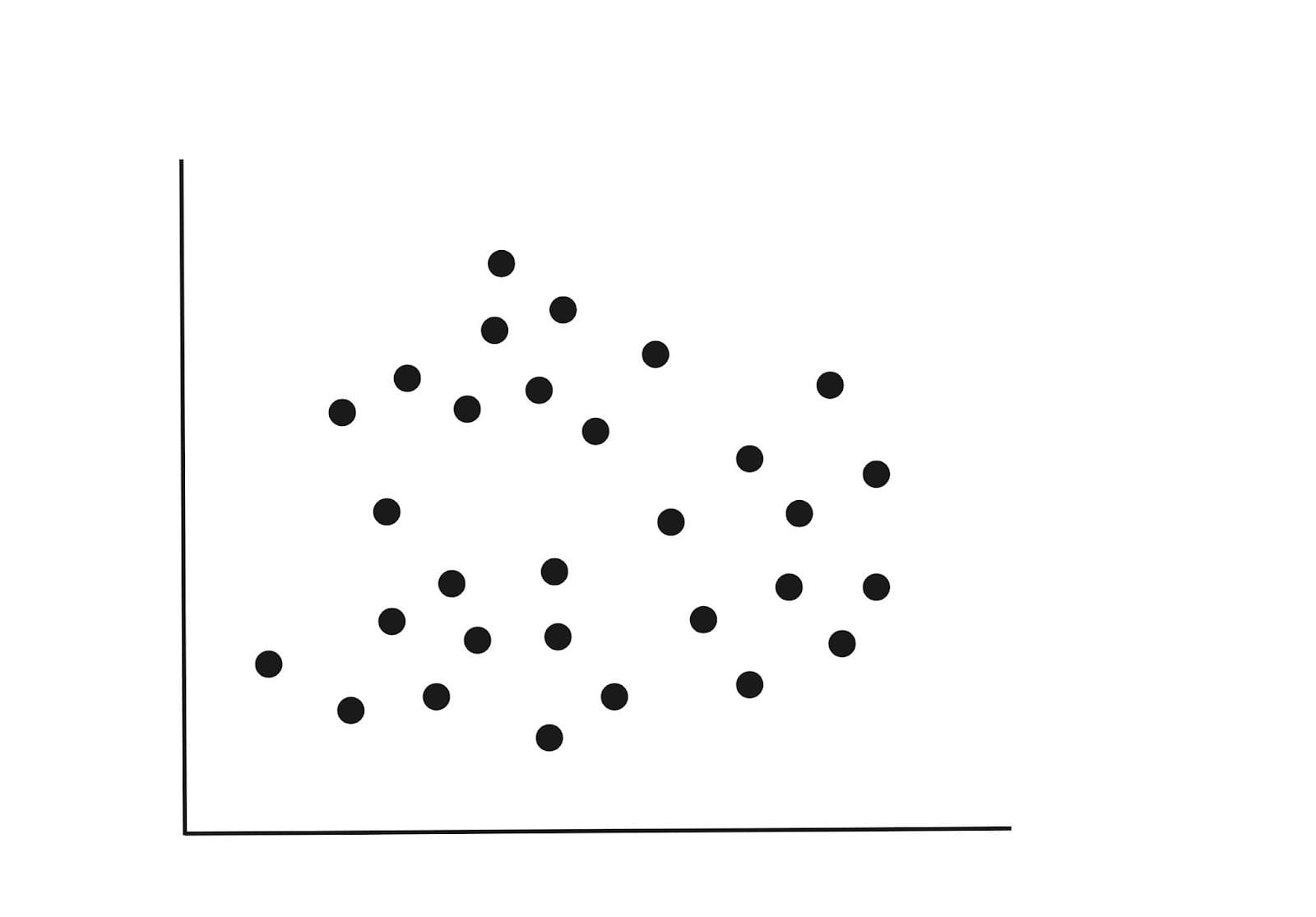
Imagine a dataset with two variables plotted as below. The variables could be the height and weight of individuals. If we had a third variable like age, then we would have a 3-D diagram, but for now, let’s stick to the 2-D diagram below.

Step 1 : Initialization
From the above diagram we can spot three clusters. When fitting our model, we can randomly assign k=3. This simply means we are seeking to split the data points into three groupings.
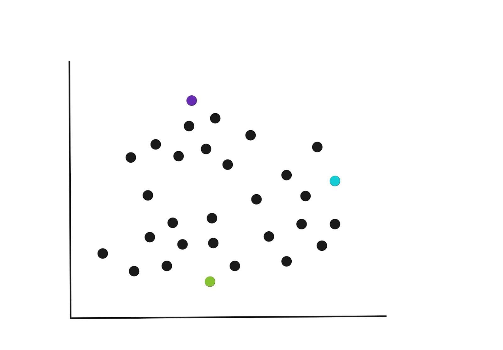
In the initial iteration, the K centroids are randomly selected in the example below.

You can specify the number of K-Clusters that the algorithm should group the data points into, however, there’s a better approach to this. We’ll dive into how to choose K later.
Step 2 : Assign points to the one of the K centroids
Once the centroids have been selected, each data point is assigned to the closest centroid, based on the euclidean distance of the point to the closest centroid. This could result in the groupings shown in the graph below.
Note that other types of distance measures can be used as manhattan distance, spearman correlation distance, and Pearson correlations distance as an alternative to euclidean, but the classical ones are euclidean and manhattan.

Step 3 : Recompute the centroids
After the first round of groupings, new centre points are recalculated again and this will necessitate a re-assignment of the points. The graph below gives an example of how the new groupings could potentially be, and notice how some points have been moved into new clusters.

Iterate
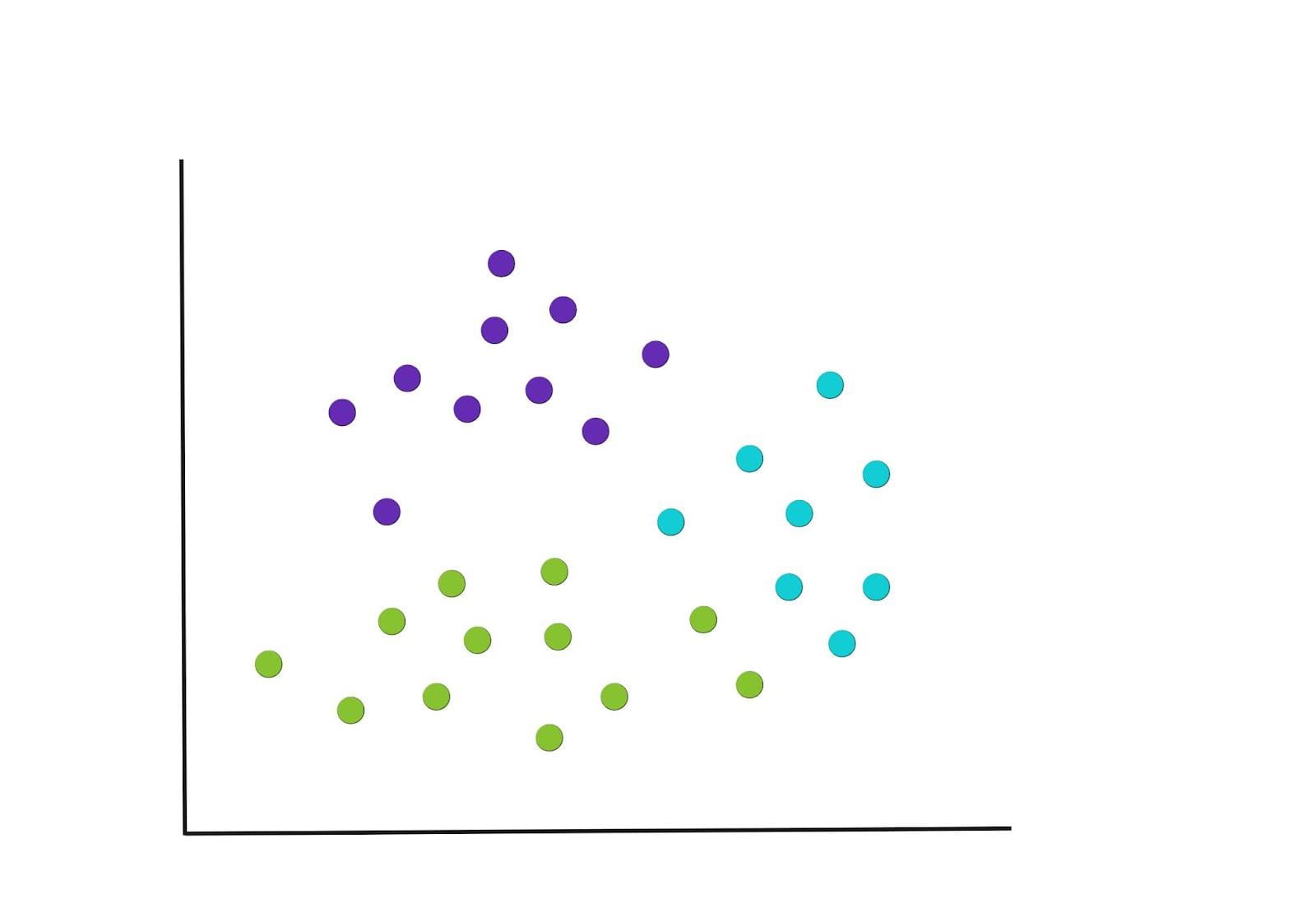
The process in steps 2 and 3 is repeated until we get to a point where there are no more reassignments of the data points or we reach the maximum number of iterations. The resulting final groupings are below.

The choice of K
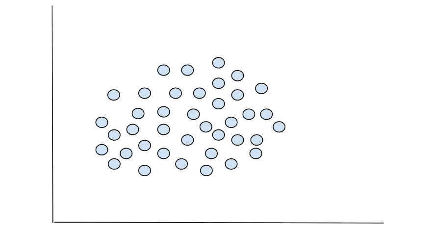
The data you will be working on as a data scientist won’t always have distinct demarcations when plotted, as you’d see on iris dataset. Oftentimes, you’ll deal with data with higher dimensions that cannot be plotted, or even if it’s plotted, you won’t be able to tell the optimum number of groupings. A good example of this is in the graph below.

Can you tell the number of groupings? Not clearly. So, how will we find the optimum number of clusters into which the above data points can be grouped?
There are different methods used to find the optimum K, into which the data points of a given data set can be grouped, elbow and silhouette methods. Let’s briefly look at how the two approaches work.
Elbow method
This approach uses the total variations within a cluster, otherwise known as the WCSS (within cluster sum of squares). The aim is to have the minimal variance within clusters (WCSS).
This method works in this way:
- It takes a range of K values, say 1 – 8 and calculates the WSS for each K value.
- The resulting data will have a K value and the corresponding WSS. This data is then used to plot a graph of WCSS against the k values.
- The optimum number of K is at the elbow point, where the curve begins to accelerate. It is from this point that the method derives its name. Think of the elbow of your arm.
Silhouette method
This method measures similarity and dissimilarity. It quantifies the distance of a point to other members of its assigned cluster, and also the distance to the members in other clusters. It works in this way:
- It takes a range of K values beginning with 2.
- For each value of K, it computes the cluster similarity, which is the average distance between a data point and all other group members in the same cluster.
- Next, the cluster dissimilarity is calculated by calculating the average distance between a data point and all other members of the nearest cluster.
- The silhouette coefficient will be the difference between cluster similarity value and cluster dissimilarity value, divided by the largest of the two values.
The optimum K would be one with the highest coefficient. The values of this coefficient are bounded in the range of -1 to 1.
Conclusion
This is an introductory article to K-Means clustering algorithm where we’ve covered what it is, how it works, and how to choose K. In the next article, we’ll walk through the process on how to solve a real world clustering problems using Python’s scikit-learn library.
Clinton Oyogo Clinton believes that analyzing data for actionable insights is a crucial part of his day-to-day work. With his skills in data visualization, data wrangling, and machine learning, he takes pride in his work as a data scientist.
Original. Reposted with permission.
- Centroid Initialization Methods for k-means Clustering
- What is Clustering and How Does it Work?
- Choosing the Right Clustering Algorithm for Your Dataset
- DBSCAN Clustering Algorithm in Machine Learning
- Key Data Science Algorithms Explained: From k-means to k-medoids clustering
- Data Versioning: Does it mean what you think it means?