Text-to-Music Generative AI : Stability Audio, Google’s MusicLM and More

Music, an art form that resonates with the human soul, has been a constant companion of us all. Creating music using artificial intelligence began several decades ago. Initially, the attempts were simple and intuitive, with basic algorithms creating monotonous tunes. However, as technology advanced, so did the complexity and capabilities of AI music generators, paving the way for deep learning and Natural Language Processing (NLP) to play pivotal roles in this tech.

Today platforms like Spotify are leveraging AI to fine-tune their users' listening experiences. These deep-learning algorithms dissect individual preferences based on various musical elements such as tempo and mood to craft personalized song suggestions. They even analyze broader listening patterns and scour the internet for song-related discussions to build detailed song profiles.

The Origin of AI in Music: A Journey from Algorithmic Composition to Generative Modeling

In the early stages of AI mixing in the music world, spanning from the 1950s to the 1970s, the focus was primarily on algorithmic composition. This was a method where computers used a defined set of rules to create music. The first notable creation during this period was the Illiac Suite for String Quartet in 1957. It used the Monte Carlo algorithm, a process involving random numbers to dictate the pitch and rhythm within the confines of traditional musical theory and statistical probabilities.

Image generated by the author using Midjourney

Image generated by the author using Midjourney

During this time, another pioneer, Iannis Xenakis, utilized stochastic processes, a concept involving random probability distributions, to craft music. He used computers and the FORTRAN language to connect multiple probability functions, creating a pattern where different graphical representations corresponded to diverse sound spaces.

The Complexity of Translating Text into Music

Music is stored in a rich and multi-dimensional format of data that encompasses elements such as melody, harmony, rhythm, and tempo, making the task of translating text into music highly complex. A standard song is represented by nearly a million numbers in a computer, a figure significantly higher than other formats of data like image, text, etc.

The field of audio generation is witnessing innovative approaches to overcome the challenges of creating realistic sound. One method involves generating a spectrogram, and then converting it back into audio.

Another strategy leverages the symbolic representation of music, like sheet music, which can be interpreted and played by musicians. This method has been digitized successfully, with tools like Magenta's Chamber Ensemble Generator creating music in the MIDI format, a protocol that facilitates communication between computers and musical instruments.

While these approaches have advanced the field, they come with their own set of limitations, underscoring the complex nature of audio generation.

Transformer-based autoregressive models and U-Net-based diffusion models, are at the forefront of technology, producing state-of-the-art (SOTA) results in generating audio, text, music, and much more. OpenAI's GPT series and almost all other LLMs currently are powered by transformers utilizing either encoder, decoder, or both architectures. On the art/image side, MidJourney, Stability AI, and DALL-E 2 all leverage diffusion frameworks. These two core technologies have been key in achieving SOTA results in the audio sector as well. In this article, we will delve into Google's MusicLM and Stable Audio, which stand as a testament to the remarkable capabilities of these technologies.

Google's MusicLM

Google's MusicLM was released in May this year. MusicLM can generate high-fidelity music pieces, that resonate with the exact sentiment described in the text. Using hierarchical sequence-to-sequence modeling, MusicLM has the capability to transform text descriptions into music that resonates at 24 kHz over extended durations.

The model operates on a multi-dimensional level, not just adhering to the textual inputs but also demonstrating the ability to be conditioned on melodies. This means it can take a hummed or whistled melody and transform it according to the style delineated in a text caption.

Technical Insights

The MusicLM leverages the principles of AudioLM, a framework introduced in 2022 for audio generation. AudioLM synthesizes audio as a language modeling task within a discrete representation space, utilizing a hierarchy of coarse-to-fine audio discrete units, also known as tokens. This approach ensures high-fidelity and long-term coherence over substantial durations.

To facilitate the generation process, MusicLM extends the capabilities of AudioLM to incorporate text conditioning, a technique that aligns the generated audio with the nuances of the input text. This is achieved through a shared embedding space created using MuLan, a joint music-text model trained to project music and its corresponding text descriptions close to each other in an embedding space. This strategy effectively eliminates the need for captions during training, allowing the model to be trained on massive audio-only corpora.

MusicLM model also uses SoundStream as its audio tokenizer, which can reconstruct 24 kHz music at 6 kbps with impressive fidelity, leveraging residual vector quantization (RVQ) for efficient and high-quality audio compression.

An illustration of the independent pretraining process for the foundational models of MusicLM: SoundStream, w2v-BERT, and MuLan,

An illustration of the pretraining process of MusicLM: SoundStream, w2v-BERT, and Mulan | Image source: here

Moreover, MusicLM expands its capabilities by allowing melody conditioning. This approach ensures that even a simple hummed tune can lay the foundation for a magnificent auditory experience, fine-tuned to the exact textual style descriptions.

The developers of MusicLM have also open-sourced MusicCaps, a dataset featuring 5.5k music-text pairs, each accompanied by rich text descriptions crafted by human experts. You can check it out here: MusicCaps on Hugging Face.

Ready to create AI soundtracks with Google's MusicLM? Here's how to get started:

  1. Visit the official MusicLM website and click “Get Started.”
  2. Join the waitlist by selecting “Register your interest.”
  3. Log in using your Google account.
  4. Once granted access, click “Try Now” to begin.

Below are a few example prompts I experimented with:

https://www.unite.ai/wp-content/uploads/2023/09/audio.wav

“Meditative song, calming and soothing, with flutes and guitars. The music is slow, with a focus on creating a sense of peace and tranquility.”

https://www.unite.ai/wp-content/uploads/2023/09/jazz-with-saxophone.wav

“jazz with saxophone”

When compared to previous SOTA models such as Riffusion and Mubert in a qualitative evaluation, MusicLM was preferred more over others, with participants favorably rating the compatibility of text captions with 10-second audio clips.

MusicLM Performance comparision

MusicLM Performance, Image source: here

Stability Audio

Stability AI last week introduced “Stable Audio” a latent diffusion model architecture conditioned on text metadata alongside audio file duration and start time. This approach like Google's MusicLM has control over the content and length of the generated audio, allowing for the creation of audio clips with specified lengths up to the training window size.

Stable Audio

Stable Audio

Technical Insights

Stable Audio comprises several components including a Variational Autoencoder (VAE) and a U-Net-based conditioned diffusion model, working together with a text encoder.

An illustration showcasing the integration of a variational autoencoder (VAE), a text encoder, and a U-Net-based conditioned diffusion model

Stable Audio Architecture, Image source: here

The VAE facilitates faster generation and training by compressing stereo audio into a data-compressed, noise-resistant, and invertible lossy latent encoding, bypassing the need to work with raw audio samples.

The text encoder, derived from a CLAP model, plays a pivotal role in understanding the intricate relationships between words and sounds, offering an informative representation of the tokenized input text. This is achieved through the utilization of text features from the penultimate layer of the CLAP text encoder, which are then integrated into the diffusion U-Net through cross-attention layers.

An important aspect is the incorporation of timing embeddings, which are calculated based on two properties: the start second of the audio chunk and the total duration of the original audio file. These values, translated into per-second discrete learned embeddings, are combined with the prompt tokens and fed into the U-Net’s cross-attention layers, empowering users to dictate the overall length of the output audio.

The Stable Audio model was trained utilizing an extensive dataset of over 800,000 audio files, through collaboration with stock music provider AudioSparx.

Stable audio commercials

Stable audio Commercials

Stable Audio offers a free version, allowing 20 generations of up to 20-second tracks per month, and a $12/month Pro plan, permitting 500 generations of up to 90-second tracks.

Below is an audio clip that I created using stable audio.

Image generated by the author using Midjourney

Image generated by the author using Midjourney

“Cinematic, Soundtrack Gentle Rainfall, Ambient, Soothing, Distant Dogs Barking, Calming Leaf Rustle, Subtle Wind, 40 BPM”

https://www.unite.ai/wp-content/uploads/2023/09/cinematic-soundtrack-gentle-rainfall-ambient-soothing-distant-dogs-barking-calming-leaf-rustle-subtle-wind-40-bpm_091623.mp3

The applications of such finely crafted audio pieces are endless. Filmmakers can leverage this technology to create rich and immersive soundscapes. In the commercial sector, advertisers can utilize these tailored audio tracks. Moreover, this tool opens up avenues for individual creators and artists to experiment and innovate, offering a canvas of unlimited potential to craft sound pieces that narrate stories, evoke emotions, and create atmospheres with a depth that was previously hard to achieve without a substantial budget or technical expertise.

Prompting Tips

Craft the perfect audio using text prompts. Here's a quick guide to get you started:

  1. Be Detailed: Specify genres, moods, and instruments. For eg: Cinematic, Wild West, Percussion, Tense, Atmospheric
  2. Mood Setting: Combine musical and emotional terms to convey the desired mood.
  3. Instrument Choice: Enhance instrument names with adjectives, like “Reverberated Guitar” or “Powerful Choir”.
  4. BPM: Align the tempo with the genre for a harmonious output, such as “170 BPM” for a Drum and Bass track.

Closing Notes

Image generated by the author using Midjourney

Image generated by the author using Midjourney

In this article, we have delved into AI-generated music/audio, from algorithmic compositions to the sophisticated generative AI frameworks of today like Google's MusicLM and Stability Audio. These technologies, leveraging deep learning and SOTA compression models, not only enhance music generation but also fine-tune listeners' experiences.

Yet, it is a domain in constant evolution, with hurdles like maintaining long-term coherence and the ongoing debate on the authenticity of AI-crafted music challenging the pioneers in this field. Just a week ago, the buzz was all about an AI-crafted song channeling the styles of Drake and The Weeknd, which had initially caught fire online earlier this year. However, it faced removal from the Grammy nomination list, showcasing the ongoing debate surrounding the legitimacy of AI-generated music in the industry (source). As AI continues to bridge gaps between music and listeners, it is surely promoting an ecosystem where technology coexists with art, fostering innovation while respecting tradition.


Using SQL to Understand Data Science Career Trends

Using SQL to Understand Data Science Career Trends
Image by Author

In a world where data is the new oil, understanding the nuances of a career in data science is more important than ever. Whether you are a data enthusiast looking or a veteran exploring opportunities, using SQL can offer insights into the data science job market.

I hope you are eager to know which data science job titles are the most attractive, or which ones offer the beefiest paychecks. Or perhaps, you're wondering how experience levels tie into data science average salaries?

In this article, we have got all those questions (and more) covered as we go deep into the data science job market. Let’s start!

Dataset Salary Trend

The dataset that we will use in this article is designed to shed light on salary patterns in the Data Science field from 2021 to 2023. By spotlighting elements such as work history, job positions, and corporate locations, it offers crucial insights into wage dispersion in the sector.

This article will find an answer to the following questions:

  1. What Does the Average Salary Look Like Across Different Experience Levels?
  2. What are the Most Common Job Titles in Data Science?
  3. How Does Salary Distribution Vary with Company Size?
  4. Where are Data Science Jobs Primarily Located Geographically?
  5. Which Job Titles Offer the Top Salaries in Data Science?

You can download this data from the Kaggle.

1. What Does the Average Salary Look Like Across Different Experience Levels?

In this SQL query, we are finding the average salary for different experience levels. The GROUP BY clause groups the data by experience level and the AVG function calculates the average salary for each group.

This helps to understand how experience in the field influences the earning potential, which is essential for you while planning your career paths in data science. Let’s see the code.

SELECT experience_level, AVG(salary_in_usd) AS avg_salary  FROM salary_data  GROUP BY experience_level;

Now let’s visualize this output by using Python.

Here is the code.

# Import required libraries for plotting  import matplotlib.pyplot as plt  import seaborn as sns  # Set up the style for the graphs  sns.set(style="whitegrid")    # Initialize the list for storing graphs  graphs = []    plt.figure(figsize=(10, 6))  sns.barplot(x='experience_level', y='salary_in_usd', data=df, estimator=lambda x: sum(x) / len(x))  plt.title('Average Salary by Experience Level')  plt.xlabel('Experience Level')  plt.ylabel('Average Salary (USD)')  plt.xticks(rotation=45)  graphs.append(plt.gcf())  plt.show()

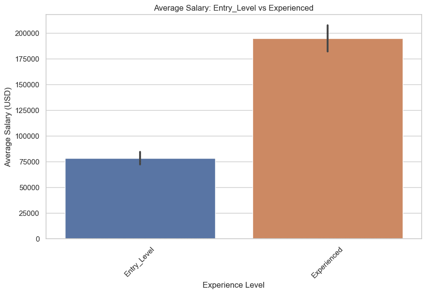
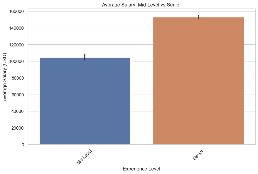
Now let’s compare, entry-level & experienced and mid-level & senior salaries.

Let’s start with entry-level & experienced. Here is the code.

# Filter the data for Entry_Level and Experienced levels  entry_experienced = df[df['experience_level'].isin(['Entry_Level', 'Experienced'])]    # Filter the data for Mid-Level and Senior levels  mid_senior = df[df['experience_level'].isin(['Mid-Level', 'Senior'])]    # Plotting the Entry_Level vs Experienced graph  plt.figure(figsize=(10, 6))  sns.barplot(x='experience_level', y='salary_in_usd', data=entry_experienced, estimator=lambda x: sum(x) / len(x) if len(x) != 0 else 0)  plt.title('Average Salary: Entry_Level vs Experienced')  plt.xlabel('Experience Level')  plt.ylabel('Average Salary (USD)')  plt.xticks(rotation=45)  graphs.append(plt.gcf())  plt.show()  

Here is the graph.

Using SQL to Understand Data Science Career Trends

Now let’s draw, mid-level & senior. Here is the code.

# Plotting the Mid-Level vs Senior graph  plt.figure(figsize=(10, 6))  sns.barplot(x='experience_level', y='salary_in_usd', data=mid_senior, estimator=lambda x: sum(x) / len(x) if len(x) != 0 else 0)  plt.title('Average Salary: Mid-Level vs Senior')  plt.xlabel('Experience Level')  plt.ylabel('Average Salary (USD)')  plt.xticks(rotation=45)  graphs.append(plt.gcf())  plt.show()  

Using SQL to Understand Data Science Career Trends

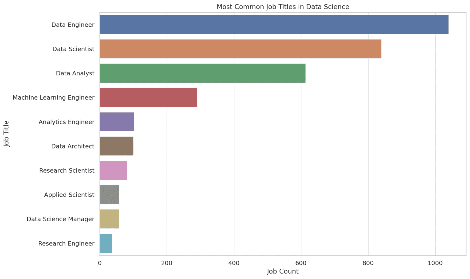
2. What are the Most Common Job Titles in Data Science?

Here, we extract the top 10 most common job titles in data science. The COUNT function counts the number of occurrences of each job title, and the results are ordered in descending order to get the most common titles at the top.

This information gives you a sense of the job market demand, guiding you in identifying potential roles you can target. Let’s see the code.

SELECT job_title, COUNT(*) AS job_count  FROM salary_data  GROUP BY job_title  ORDER BY job_count DESC  LIMIT 10;

Okay, it is time to visualize this query by using Python.

Here is the code.

plt.figure(figsize=(12, 8))  sns.countplot(y='job_title', data=df, order=df['job_title'].value_counts().index[:10])  plt.title('Most Common Job Titles in Data Science')  plt.xlabel('Job Count')  plt.ylabel('Job Title')  graphs.append(plt.gcf())  plt.show()

Let’s see the graph.

Using SQL to Understand Data Science Career Trends

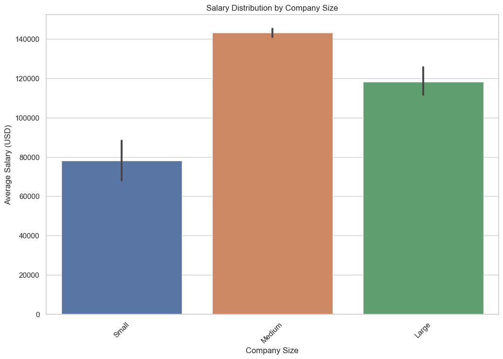
3. How Does Salary Distribution Vary with Company Size?

In this query, we extract the average, minimum, and maximum salaries for each company size grouping. Using aggregate functions such as AVG, MIN, and MAX helps to provide a comprehensive view of the salary landscape in relation to the size of a company.

This data is essential as it helps you understand the potential earnings you can expect depending on the size of the company you are looking to join, let’s see the code.

SELECT company_size, AVG(salary_in_usd) AS avg_salary, MIN(salary_in_usd) AS min_salary, MAX(salary_in_usd) AS max_salary  FROM salary_data  GROUP BY company_size;

Now let’s visualize this query, by using Python.

Here is the code.

plt.figure(figsize=(12, 8))  sns.barplot(x='company_size', y='salary_in_usd', data=df, estimator=lambda x: sum(x) / len(x) if len(x) != 0 else 0, order=['Small', 'Medium', 'Large'])  plt.title('Salary Distribution by Company Size')  plt.xlabel('Company Size')  plt.ylabel('Average Salary (USD)')  plt.xticks(rotation=45)  graphs.append(plt.gcf())  plt.show()

Here is the output.

Using SQL to Understand Data Science Career Trends

4. Where are Data Science Jobs Primarily Located Geographically?

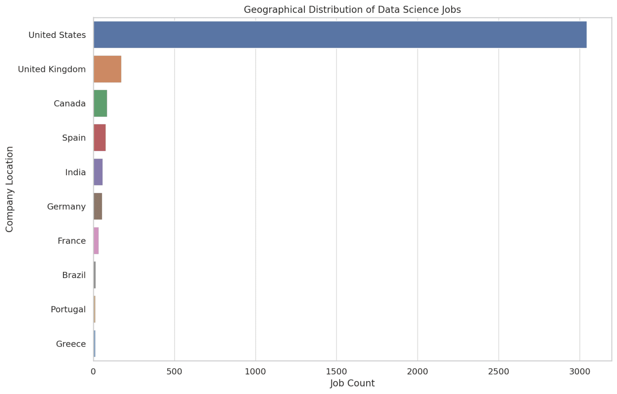
Here, we pinpoint the top 10 locations holding the highest number of data science job opportunities. We use the COUNT function to determine the number of job postings in each location, arranging them in descending order to spotlight the areas with the most opportunities.

Having this information equips readers with knowledge of the geographical areas that are hubs for data science roles, aiding in potential relocation decisions. Let’s see the code.

SELECT company_location, COUNT(*) AS job_count  FROM salary_data  GROUP BY company_location  ORDER BY job_count DESC  LIMIT 10;

Now let’s create graphs of the code above, with Python.

plt.figure(figsize=(12, 8))  sns.countplot(y='company_location', data=df, order=df['company_location'].value_counts().index[:10])  plt.title('Geographical Distribution of Data Science Jobs')  plt.xlabel('Job Count')  plt.ylabel('Company Location')  graphs.append(plt.gcf())  plt.show()

Let’s see the graph below.

Using SQL to Understand Data Science Career Trends

5. Which Job Titles Offer the Top Salaries in Data Science?

Here, we are identifying the top 10 highest-paying job titles in the data science sector. By using the AVG, we calculate the average salary for each job title, sorting them in descending order based on the average salary to highlight the most lucrative positions.

You can aspire to in your career journey, by looking at this data. Let’s proceed to understand how readers can create a Python visualization for this data.

SELECT job_title, AVG(salary_in_usd) AS avg_salary  FROM salary_data  GROUP BY job_title  ORDER BY avg_salary DESC  LIMIT 10;

Here is the output.

(Here we can not use photos, because we added 4 photos above, and one left for a thumbnail, Do we have a chance to use a table like below to demonstrate the output?)

Rank Job Title Average Salary (USD)
1 Data Science Tech Lead 375,000.00
2 Cloud Data Architect 250,000.00
3 Data Lead 212,500.00
4 Data Analytics Lead 211,254.50
5 Principal Data Scientist 198,171.13
6 Director of Data Science 195,140.73
7 Principal Data Engineer 192,500.00
8 Machine Learning Software Engineer 192,420.00
9 Data Science Manager 191,278.78
10 Applied Scientist 190,264.48

This time, let’s try to create a graph by yourself.

Tips: You can use the following prompt in ChatGPT to generate a Pythonic code of this graph:

<SQL Query here>    Create a Python graph to visualize the top 10 highest-paying job titles in Data Science, similar to the insights gathered from the given SQL query above.

Final Thoughts

As we wrap up our journey through the diverse terrains of the data science career world, we hope SQL proves to be a trustworthy guide, helping you unearth gems of insights to support your career decisions.

I hope that you feel more equipped now, not just in mapping your career path, but also in using SQL in shaping raw data into powerful narratives. So here's to stepping into a future filled with opportunities, with data as your compass and SQL as your guiding force!

Thanks for reading!
Nate Rosidi is a data scientist and in product strategy. He's also an adjunct professor teaching analytics, and is the founder of StrataScratch, a platform helping data scientists prepare for their interviews with real interview questions from top companies. Connect with him on Twitter: StrataScratch or LinkedIn.

More On This Topic

  • Using Twitter to Understand Pizza Delivery Apprehension During COVID
  • Data Science and Analytics Career Trends for 2021
  • 5 Key Data Science Trends & Analytics Trends
  • Graphs: The natural way to understand data
  • 24 Best (and Free) Books To Understand Machine Learning
  • Picking Examples to Understand Machine Learning Model

Why IT growth is only leading to more burnout, and what should be done about it

burnout

While information technology work — development, engineering, administration, hand-holding — is considered among the world's most preferable jobs, it is also a source of unending burnout. Major causes include excessive workloads, excessive hours worked, lack of recognition, and lack of challenges, explains Nick Kolakowski in a recent Dice report.

Let's look closer at those first two factors — excessive workloads and hours. While there are many activities tech professionals need to pursue all at once, one thing that clogs their days up more than anything is the overwhelming number of glitches, outages, breaches, and other incidents that demand their attention.

Also: Can Microsoft recover from the collapse of its Surface business?

When systems glitch, end users and customers can get extremely frustrated. They wonder: isn't anyone minding the store? The answer, of course, is there are IT teams minding the store. But they're getting just as frustrated as anyone else dealing with issues that arise.

Business' leaders ought to be frustrated, too, because there's a real cost to their organizations as well. Incidents can cost large companies more than $100 million a year, according to a recent analysis and survey out of Constellation Research. "Even more eye-opening, 49% of those incidents are straightforward and repetitive, and can be automated away," the report's author, Andy Thurai of Constellation Research, observes.

Also: OpenAI announces first developer conference: Everything we know so far

More than half of 317 IT managers responding to the Constellation survey, 57%, indicate that they get more incidents than they can handle. "This is alarming, especially because the number of incidents is continuing to increase and incident response teams are already overwhelmed," according to Thurai. "Poor incident response experience with repetitive, manual toil can lead to employee attrition. In fact, it is cited as the top cause of employee attrition by many incident responders."

Add a lack of organizational support and awareness to the mix. "Leadership lacks visibility into top incidents, team toil, team burnout, and incident response costs," Thurai observes. "Continuing with older practices leads to too many alerts, creating alert fatigue."

While there are some robust tools and platforms on the market that help automate and alleviate this pain, the growth of cloud, analytics, and distributed systems has made incident response only more complex. "Incidents, both major and minor, are more frequent than expected," the survey shows. Plus, "the current way of responding to incidents is broken."

There has been some progress in the five years since Constellation's previous survey on this topic. In both cases, more than one-third report more than five major incidents within the past 12 months with their production cloud infrastructures. (Thirty-four percent this year, down slightly from 38% five years ago.)

Also: My two favorite ChatGPT Plus plugins and the remarkable things I can do with them

"In other words, companies have not reduced the rate of major incidents with their production cloud infrastructure," Thurai, points out. He cites rising rates of cloud adoption and newer applications in deployment, and the continued prevalence of manual processes to respond to IT incidents. Couple that with a shortage of skilled IT personnel, who are already overwhelmed with multiple demands.

IT managers are almost unanimous that something needs to be done, the Constellation survey shows. Nine in ten agree that companies with a high degree of automation have the most effective incident response. The same number state that "application downtime is a top cause of customer dissatisfaction and churn."

Some of the actions Thurai recommends to reduce burnout and alert fatigue include the following:

  • Automate as much as possible. This should ultimately include self-healing capabilities. "They can be pre- or post-automation remediation measures to avoid incidents."
  • Educate and train: Help IT staff become "more knowledgeable so they can solve incidents without escalating."
  • Get the business on board: "Every board member should be asking these questions of their IT executives: If a major incident happened to us, how would you manage it? Would we be able to handle it and prove to our customers that we are worthy of their trust, or would we botch it and cease to exist? If we are not prepared now, how can we get prepared? Ask for a plan of action and proof. Be willing to fund what's necessary to make this happen."
  • Take a team approach: Thurai advocates for the "automated creation of collaboration or war rooms," as well as the "immediate creation of conference or video call links associated with the incident to reduce the need for manual intervention and save valuable time during major incidents."

Just as important as these more direct actions to address incident fatigue is providing a rewarding, meaningful, and — yes, I'll say it — fun workplace atmosphere for all levels of professionals. It's time to recognize the hard work that goes into building digital businesses.

Featured

Top 5 Libraries in C/C++ for ML in 2023

Being a compiled language, C++, the go-to framework for developers, can translate into machine code before execution, making it ideal for computationally intensive jobs like training large neural networks. Its robust memory management provides optimisation opportunities for machine learning algorithms.

Moreover, it seamlessly integrates with other tools such as CUDA and OpenCL, enabling GPU-based computing, which significantly enhances deep learning tasks’ speed. There are tons of such libraries available such as TensorFlow, Caffe, and mlpack. Let’s take a look at some of the C/C++ libraries for machine learning.

Read more: Should Developers Choose C++ Over Python for Machine Learning?

OpenCV

OpenCV, short for Open Source Computer Vision, is a widely recognised C library known for its versatility and robustness. Supported by high-level programming languages such as Java and Python, it seamlessly integrates with deep learning frameworks like TensorFlow, Torch, and PyTorch. This open-source package boasts a comprehensive collection of over 2,500 optimised algorithms, catering to various functions such as face recognition, object detection, 3D model extraction, and more.

Originally initiated by Intel in 1999, it has gained cross-platform compatibility, with interfaces for C++, Python, Java, and MATLAB, and supports Windows, Linux, Android, and Mac OS. Despite its C foundation, OpenCV remains a go-to choice for machine learning and computer vision applications, making it a popular tool with over 29,000 weekly downloads. MobileNets + Single Shot Detectors and YoloV5 are based on OpenCV.

FAISS

Facebook AI Similarity Search (FAISS) is a powerful library for swiftly discovering similar multimedia documents, excelling with datasets of billions of examples and offering an impressive 8.5 times speed boost compared to the fastest k-sampling GPU algorithm. Developed by Facebook AI Research, Faiss is a C++ tool optimized for efficient similarity search and clustering of dense vectors. It delivers diverse similarity search methods, is highly parallelizable for multi-core and multi-GPU utilisation, and comes with Python wrappers.

Faiss is open source, residing on GitHub, and includes code for evaluation and parameter tuning. It accommodates datasets of any size, even those exceeding RAM capacity, drawing from extensive research. Notably, Faiss outpaces Scikit-Learn by 20 times in k-means clustering speed. However, it’s essential to consider its suitability for specific machine-learning tasks.

Scikit-Learn

Scikit-Learn is a robust Python library built on NumPy and SciPy, serving as a valuable tool for data preprocessing and modelling tasks encompassing supervised and unsupervised learning. With an active and supportive community, it offers solutions to various queries. Its versatile applications include decision trees, linear and logistic regression, classification, clustering, and SVM, particularly in data preprocessing, hash vectorization, and TF-IDF. However, it’s not designed for large-scale production environments. Random Forest Classifiers, Support Vector Machines (SVM), K-Means Clustering, and Gradient Boosting are based on this.

Scipy

A scientific computing library for Python, SciPy offers modules for optimization, linear algebra, integration, interpolation, signal and image processing, and more, with C and C++ interfaces. While it’s not explicitly tailored for machine learning, it can still be applied in tasks like data preprocessing and feature extraction. It stands as one of the top machine learning libraries in C++, serving scientific, engineering, and commercial projects due to its robust support for natural language processing. SciPy builds upon the popular NumPy library, extending its capabilities to encompass tasks like Fourier transforms, image optimization, integration, interpolation, differential equation solving, and more, offering valuable packages like cluster, fft, interpolates, and ndimage.

Armadillo

Armadillo is a C++ library known for its proficiency in linear algebra and scientific computations, boasting strong performance, seamless integration with C++ code, a user-friendly API, and open-source accessibility. While it isn’t a full-fledged machine learning library, it excels at efficient linear algebra tasks, making it an attractive choice for C++ developers requiring swift mathematical computations. For comprehensive machine learning endeavours, it’s common to combine Armadillo with specialised libraries like TensorFlow, PyTorch, or Scikit-Learn to handle broader machine learning functionalities.

In addition to linear algebra, Armadillo provides a rich toolkit for managing vectors, matrices, and cubes, featuring a robust expression parser, adaptive matrix evaluation, diverse matrix decomposition techniques, OpenMP multi-threading support, and more. These capabilities collectively position Armadillo as an excellent option for developing applications across various domains, including machine learning, pattern recognition, computer vision (with a particular emphasis on medical applications), signal processing, statistics, and beyond.

The post Top 5 Libraries in C/C++ for ML in 2023 appeared first on Analytics India Magazine.

Building a Convolutional Neural Network with PyTorch

Building a Convolutional Neural Network with PyTorch
Image by Author Introduction

A Convolutional Neural Network (CNN or ConvNet) is a deep learning algorithm specifically designed for tasks where object recognition is crucial — like image classification, detection, and segmentation. CNNs are able to achieve state-of-the-art accuracy on complex vision tasks, powering many real-life applications such as surveillance systems, warehouse management, and more.

As humans, we can easily recognize objects in images by analyzing patterns, shapes, and colors. CNNs can be trained to perform this recognition too, by learning which patterns are important for differentiation. For example, when trying to distinguish between a photo of a Cat versus a Dog, our brain focuses on unique shape, textures, and facial features. A CNN learns to pick up on these same types of distinguishing characteristics. Even for very fine-grained categorization tasks, CNNs are able to learn complex feature representations directly from pixels.

In this blog post, we will learn about Convolutional Neural Networks and how to use them to build an image classifier with PyTorch.

How Convolutional Neural Networks Work?

Convolutional neural networks (CNNs) are commonly used for image classification tasks. At a high level, CNNs contain three main types of layers:

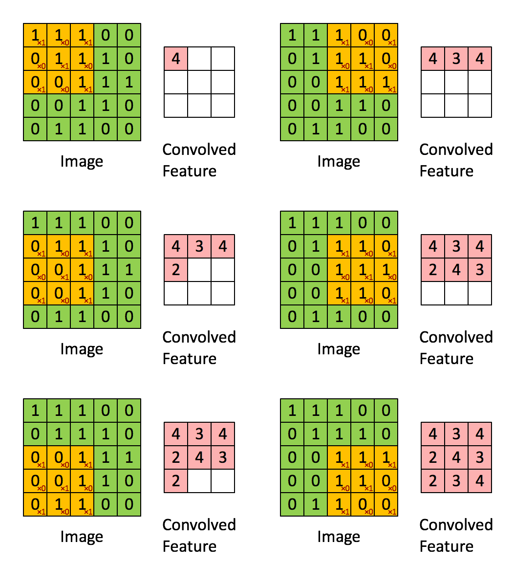
  1. Convolutional layers. Apply convolutional filters to the input to extract features. The neurons in these layers are called filters and capture spatial patterns in the input.
  2. Pooling layers. Downsample the feature maps from the convolutional layers to consolidate information. Max pooling and average pooling are commonly used strategies.
  3. Fully-connected layers. Take the high-level features from the convolutional and pooling layers as input for classification. Multiple fully-connected layers can be stacked.

The convolutional filters act as feature detectors, learning to activate when they see specific types of patterns or shapes in the input image. As these filters are applied across the image, they produce feature maps that highlight where certain features are present.

For example, one filter might activate when it sees vertical lines, producing a feature map showing the vertical lines in the image. Multiple filters applied to the same input produce a stack of feature maps, capturing different aspects of the image.

Building a Convolutional Neural Network with PyTorch
Gif by IceCream Labs

By stacking multiple convolutional layers, a CNN can learn hierarchies of features — building up from simple edges and patterns to more complex shapes and objects. The pooling layers help consolidate the feature representations and provide translational invariance.

The final fully-connected layers take these learned feature representations and use them for classification. For an image classification task, the output layer typically uses a softmax activation to produce a probability distribution over classes.

In PyTorch, we can define the convolutional, pooling, and fully-connected layers to build up a CNN architecture. Here is some sample code:

# Conv layers   self.conv1 = nn.Conv2d(in_channels, out_channels, kernel_size)  self.conv2 = nn.Conv2d(in_channels, out_channels, kernel_size)    # Pooling layer  self.pool = nn.MaxPool2d(kernel_size)    # Fully-connected layers   self.fc1 = nn.Linear(in_features, out_features)  self.fc2 = nn.Linear(in_features, out_features)

We can then train the CNN on image data, using backpropagation and optimization. The convolutional and pooling layers will automatically learn effective feature representations, allowing the network to achieve strong performance on vision tasks.

Getting Started with CNNs

In this section, we will load CIFAR10 and build and train a CNN-based classification model using PyTorch. The CIFAR10 dataset provides 32×32 RGB images across ten classes, which is useful for testing image classification models. There are ten classes labeled in integers 0 to 9.

Note: The example code is the modified version from MachineLearningMastery.com blog.

First, we will use torchvision to download and load the CIFAR10 dataset. We will also use torchvision to transform both the testing and training sets to tensors.

import torch  import torch.nn as nn  import torch.optim as optim  import torchvision    transform = torchvision.transforms.Compose(      [torchvision.transforms.ToTensor()]  )    train = torchvision.datasets.CIFAR10(      root="data", train=True, download=True, transform=transform  )    test = torchvision.datasets.CIFAR10(      root="data", train=False, download=True, transform=transform  )
Downloading https://www.cs.toronto.edu/~kriz/cifar-10-python.tar.gz to data/cifar-10-python.tar.gz    100%|██████████| 170498071/170498071 [00:10<00:00, 15853600.54it/s]    Extracting data/cifar-10-python.tar.gz to data  Files already downloaded and verified

After that, we will use a data loader and split the images into the batches.

batch_size = 32  trainloader = torch.utils.data.DataLoader(      train, batch_size=batch_size, shuffle=True  )  testloader = torch.utils.data.DataLoader(      test, batch_size=batch_size, shuffle=True  )

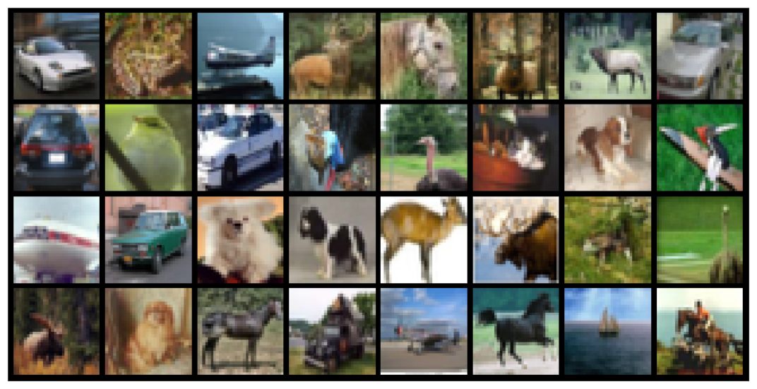
To visualize the image in a single batch of the images, we will use matplotlib and torchvision utility function.

from torchvision.utils import make_grid  import matplotlib.pyplot as plt    def show_batch(dl):      for images, labels in dl:          fig, ax = plt.subplots(figsize=(12, 12))          ax.set_xticks([]); ax.set_yticks([])          ax.imshow(make_grid(images[:64], nrow=8).permute(1, 2, 0))          break  show_batch(trainloader)

As we can see, we have images of cars, animals, planes, and boats.

Building a Convolutional Neural Network with PyTorch

Next, we will build our CNN model. For that, we have to create a Python class and initialize the convolutions, maxpool, and fully connected layers. Our architecture has 2 convolutional layers with pooling and linear layers.

After initializing, we will not connect all the layers sequentially in the forward function. If you are new to PyTorch, you should read Interpretable Neural Networks with PyTorch to understand each component in detail.

class CNNModel(nn.Module):      def __init__(self):          super().__init__()          self.conv1 = nn.Conv2d(3, 32, kernel_size=(3,3), stride=1, padding=1)          self.act1 = nn.ReLU()          self.drop1 = nn.Dropout(0.3)             self.conv2 = nn.Conv2d(32, 32, kernel_size=(3,3), stride=1, padding=1)          self.act2 = nn.ReLU()          self.pool2 = nn.MaxPool2d(kernel_size=(2, 2))             self.flat = nn.Flatten()             self.fc3 = nn.Linear(8192, 512)          self.act3 = nn.ReLU()          self.drop3 = nn.Dropout(0.5)             self.fc4 = nn.Linear(512, 10)         def forward(self, x):          # input 3x32x32, output 32x32x32          x = self.act1(self.conv1(x))          x = self.drop1(x)          # input 32x32x32, output 32x32x32          x = self.act2(self.conv2(x))          # input 32x32x32, output 32x16x16          x = self.pool2(x)          # input 32x16x16, output 8192          x = self.flat(x)          # input 8192, output 512          x = self.act3(self.fc3(x))          x = self.drop3(x)          # input 512, output 10          x = self.fc4(x)          return x

We will now initialize our model, set loss function, and optimizer.

model = CNNModel()  loss_fn = nn.CrossEntropyLoss()  optimizer = optim.SGD(model.parameters(), lr=0.001, momentum=0.9)

In the training phase, we will train our model for 10 epochs.

  1. We are using the forward function of the model for a forward pass, then a backward pass using the loss function, and finally updating the weights. This step is almost similar in all kinds of neural network models.
  2. After that, we are using a test data loader to evaluate model performance at the end of each epoch.
  3. Calculating the accuracy of the model and printing the results.
n_epochs = 10  for epoch in range(n_epochs):      for i, (images, labels) in enumerate(trainloader):          # Forward pass           outputs = model(images)          loss = loss_fn(outputs, labels)            # Backward pass and optimize          optimizer.zero_grad()          loss.backward()          optimizer.step()      correct = 0      total = 0      with torch.no_grad():          for images, labels in testloader:              outputs = model(images)              _, predicted = torch.max(outputs.data, 1)              total += labels.size(0)              correct += (predicted == labels).sum().item()        print('Epoch %d: Accuracy: %d %%' % (epoch,(100 * correct / total)))  

Our simple model has achieved 57% accuracy, which is bad. But, you can improve the model performance by adding more layers, running it for more epochs, and hyperparameter optimization.

Epoch 0: Accuracy: 41 %  Epoch 1: Accuracy: 46 %  Epoch 2: Accuracy: 48 %  Epoch 3: Accuracy: 50 %  Epoch 4: Accuracy: 52 %  Epoch 5: Accuracy: 53 %  Epoch 6: Accuracy: 53 %  Epoch 7: Accuracy: 56 %  Epoch 8: Accuracy: 56 %  Epoch 9: Accuracy: 57 %  

With PyTorch, you don't have to create all the components of convolutional neural networks from scratch as they are already available. It becomes even simpler if you use `torch.nn.Sequential`. PyTorch is designed to be modular and offers greater flexibility in building, training, and assessing neural networks.

Conclusion

In this post, we explored how to build and train a convolutional neural network for image classification using PyTorch. We covered the core components of CNN architectures — convolutional layers for feature extraction, pooling layers for downsampling, and fully-connected layers for prediction.

I hope this post provided a helpful overview of implementing convolutional neural networks with PyTorch. CNNs are fundamental architecture in deep learning for computer vision, and PyTorch gives us the flexibility to quickly build, train, and evaluate these models.

Abid Ali Awan (@1abidaliawan) is a certified data scientist professional who loves building machine learning models. Currently, he is focusing on content creation and writing technical blogs on machine learning and data science technologies. Abid holds a Master's degree in Technology Management and a bachelor's degree in Telecommunication Engineering. His vision is to build an AI product using a graph neural network for students struggling with mental illness.

More On This Topic

  • Learn Deep Learning by Building 15 Neural Network Projects in 2022
  • Building and Training Your First Neural Network with TensorFlow and Keras
  • Image Classification with Convolutional Neural Networks (CNNs)
  • A Comprehensive Guide to Convolutional Neural Networks
  • Building Multimodal Models: Using the widedeep Pytorch package
  • Don’t Waste Time Building Your Data Science Network

Elicit is building a tool to automate scientific literature review

Elicit is building a tool to automate scientific literature review Kyle Wiggers 7 hours

For researchers, reading scientific papers can be immensely time-consuming. According to one survey, scientists spend seven hours each week searching for information. Another survey suggests that systematic reviews of literature — scholarly syntheses of the evidence on a particular topic — take an average of 41 weeks for a five-person research team.

But it doesn’t have to be this way.

At least, that’s the message from Andreas Stuhlmüller, the co-founder of an AI startup, Elicit, that’s designed a “research assistant” for scientists and R&D labs. With backers including Fifty Years, Basis Set, Illusion and angel investors Jeff Dean (Google’s chief scientist) and Thomas Ebeling (the former Novartis CEO), Elicit is building an AI-powered tool to abstract away the more tedious aspects of literature review.

“Elicit is a research assistant that automates scientific research with language models,” Stuhlmüller told TechCrunch in an email interview. “Specifically, it automates literature review by finding relevant papers, extracting key information about the studies and organizing the information into concepts.”

Elicit is a for-profit venture spun out from Ought, a nonprofit research foundation launched in 2017 by Stuhlmüller, a former researcher at Stanford’s computation and cognition lab. Elicit’s other co-founder, Jungwon Byun, joined the startup in 2019 after leading growth at online lending firm Upstart.

Using a variety of models both first- and third-party, Elicit searches and discovers concepts across papers, allowing users to ask questions like “What are all of the effects of creatine?” or “What are all of the data sets that have been used to study logical reasoning?” and get a list of answers from the academic literature.

“By automating the systematic review process, we can immediately deliver cost and time savings to the academic and industry research organizations producing these reviews,” Stuhlmüller said. “By lowering the cost enough, we unlock new use cases that were previously cost-prohibitive, such as just-in-time updates when the state of knowledge in a field changes.”

But wait, you might say — don’t language models have a tendency to make things up? Indeed they do. Meta’s attempt at a language model to streamline scientific research, Galactica, was taken down only three days after launch, once it was discovered that the model frequently referred to fake research papers that sounded right but weren’t actually factual.

Stuhlmüller claims Elicit has taken steps to ensure its AI is more reliable than many of the purpose-built platforms out there, however.

For one, Elicit breaks down the complex tasks that its models perform into “human-understandable” pieces. This enables Elicit to know, for instance, how often different models are making things up when they generate summaries, and subsequently help users identify what answers to check — and when.

Elicit also attempts to compute a scientific paper’s overall “trustworthiness,” taking into account factors like whether the trials conducted in the research were controlled or randomized, the source of the funding and potential conflicts and the size of the trials.

Elicit

Elicit’s search tool for AI literature.

“We don’t do chat interfaces,” Stuhlmüller said. “Elicit users apply language models as batch jobs … We never just generate answers using models, we always link the answers back to the scientific literature to reduce hallucination and make it easy to check models’ work.”

I’m not necessarily convinced that Elicit has solved some of the major issues plaguing language models today, given their intractability. But its efforts certainly appear to have garnered interest — and perhaps even trust — from the research community.

Stuhlmüller claims that over 200,000 people are using Elicit every month, representing 3x year-over-year growth, from organizations including The World Bank, Genentech and Stanford. “Our users are asking to pay for more powerful features and to run Elicit at larger scales,” he added.

Presumably, it’s this momentum that led to Elicit’s first funding round — a $9 million tranche led by Fifty Years. The plan is to put the bulk of the new cash toward further developing Elicit’s product as well as expanding Elicit’s team of product managers and software engineers.

But what’s Elicit’s plan to make money? Good question — and one I asked Stuhlmüller point blank. He pointed to Elicit’s paid teir, launched this week, that lets users search papers, extract data and summarize concepts at a larger scale than the free tier supports. The longer-term strategy is to build Elicit into a general tool for research and reasoning — one that whole enterprises would shell out for.

One possible roadblock to Elicit’s commercial success are open source efforts like the Allen Institute for AI’s Open Language Model, which aim to develop a free-to-use large language model optimized for science. But Stuhlmüller says that he sees open source more as complementary than threatening.

“The primary competition right now is human labor — research assistants that are hired to painstakingly extract data from papers,” Stuhlmüller said. “Scientific research is a huge market and research workflow tooling has no major incumbents. This is where we’ll see entirely new AI-first workflows emerge.”

6 Brilliant JavaScript Frameworks for Every Developer

While JavaScript might not be the first choice for developing and training machine learning models, it is important for integrating ML into web applications, creating user interfaces, and deploying models on the client side. It complements Python in the machine learning ecosystem, allowing developers to build end-to-end solutions that involve both frontend and backend components.

Although Python and R are more prevalent for machine learning, Java can serve this purpose effectively, especially if you’re already proficient in it. In addition to Brains.js, Keras.js, and TensorFlow.js, we’ve compiled a selection of some important Java frameworks for machine learning, data science, data visualization, natural language processing, and other related areas. Let’s explore a few of them.

Synaptic.js

Synaptic.js, a renowned open-source neural network library in JavaScript, empowers machine learning model development and training. It boasts an architecture-agnostic nature, accommodating both first-order and second-order neural network designs. This versatile tool serves multiple purposes in machine learning like network construction and training, long short-term memory (LSTM) and recurrent neural network (RNN) capabilities, game development, predictive modelling and more.

OpenCV.js

A JavaScript binding that brings a specific subset of OpenCV functionalities to web applications, OpenCV.js empowers web-based projects with multimedia processing capabilities, tapping into OpenCV’s rich set of vision functions. OpenCV.js utilizes Emscripten to compile OpenCV functions into asm.js or WebAssembly targets, offering a JavaScript API for web apps to access these features. Its benefits include seamless browser integration, enabling easy access for internet users, multimedia processing support for emerging web applications, extending OpenCV’s reach by providing a JavaScript interface for languages beyond C and C++, and delivering high performance through ASM.js and SIMD.js, all while being freely available under a BSD license. It finds applications in image processing, feature extraction, object and face detection, camera calibration, machine learning, automated inspection, surveillance, and interactive art installations.

D3.js

D3.js, short for Data-Driven Documents, is a JavaScript library that empowers developers to craft dynamic and interactive web data visualizations. It offers a wide range of chart types, including bar charts, line charts, scatterplots, and interactive maps, while also enabling robust data tasks like filtering, binding, and manipulation. By seamlessly blending Scalable Vector Graphics (SVG) and HTML elements, D3.js facilitates the creation of highly responsive and customized data visualizations. Moreover, it boasts an array of layout algorithms for crafting intricate visualizations such as hierarchical layouts and network graphs. Predominantly utilized in journalism and academic pursuits, D3 is a versatile tool for transforming data into compelling visuals, encompassing various chart types like box plots, histograms, treemaps, chard graphs, scatter plots, line charts, bar charts, pie charts, and more. It further enhances visual appeal with animation features like animated treemaps, zoomable bar charts, icicles, and bar chart races, offering a comprehensive suite for data analysis and storytelling.

Compromise.js

Designed for natural language processing for both Node.js and browser environments, Compromise.js offers a robust toolkit for parsing, understanding, and manipulating English text, akin to NLP.js. An additional feature is its plugin system, facilitating the expansion of functionality through custom modules. With Compromise, users can effortlessly extract various text elements such as nouns, verbs, adjectives, dates, times, and addresses. Moreover, it supports text operations such as pluralization, capitalization, contractions, and expansions. It also encompasses sentiment analysis, named entity recognition, part-of-speech tagging, and verb conjugation. Notably, Compromise excels in efficiency, capable of handling nearly all English vocabulary using just 14,000 words, compressed into a compact 40kb file size. This exceptional compression enables swift text comprehension and scanning with minimal latency, measured in milliseconds.

ConvNetJS

The brainchild of deep learning genius Andrej Karpathy, ConvNetJS, is a JavaScript library, that enables users to train deep learning models, particularly neural networks, directly within their web browsers. Notably, ConvNetJS leverages the browser’s hardware acceleration capabilities, eliminating the need for specialized software like GPUs or compilers. It offers user-friendly JavaScript tools for formulating and solving neural networks, addressing various tasks, including classification, regression, image processing with convolutional networks, and experimental reinforcement learning via Deep Q Learning. Additionally, it extends support to Node.js and is open source on GitHub under the MIT license, welcoming contributions for new features and improvements. In summary, ConvNetJS serves as a potent resource for training deep learning models effortlessly within web browsers.

JSFeat

JSFeat is a JavaScript computer vision library that enables JavaScript to harness a wide range of image processing and computer vision algorithms. Its capabilities encompass tasks like edge detection, image processing (including grayscale and blur operations), corner detection, object identification, optical flow detection, and more. At the heart of JSFeat is the adaptable matrix_t structure, which serves as a versatile foundation for tasks ranging from image representation to mathematical operations. The library also incorporates an innovative linked pool-based cache system, enhancing performance by optimizing buffer allocation. In addition to the inherent benefits of JavaScript, such as speed, user-friendliness, versatility, and cross-platform compatibility, JSFeat specifically offers portability across JavaScript-supported platforms, ease of integration with other programming languages, real-time performance for demanding applications and comprehensive documentation for developer convenience.

The post 6 Brilliant JavaScript Frameworks for Every Developer appeared first on Analytics India Magazine.

NVIDIA’s Dominance Set to Surge Further

NVIDIA is poised to ascend first in the semiconductor world in 2023, as per findings from SC-IQ. The report indicates that NVIDIA is on track to achieve a remarkable revenue of nearly $53 billion in the fiscal year 2023.

The report underscores NVIDIA’s extraordinary growth, with its projected revenue for the current year nearly doubling the figures from 2022, which stood at $26.3 billion. This surge is primarily driven by the soaring demand for NVIDIA’s processors, which are instrumental in fueling the ongoing AI revolution

Revenue Estimates for Third Quarter

NVIDIA posted a revenue of $7.1 billion in Q1 2023 and an all time high of $13.5 billion in revenue in Q2 2023. Analysts estimate that Q3 will generate around $16 billion. The revenue growth from the last four quarters is 31.6% and if this trend continues, the Q4 2023 revenue would be around $18 billion. This would be a combined revenue of $54 billion for NVIDIA in 2023 if the trend continues. This number supports the prediction of the SC-IQ report.

When it comes to generating income, the company has no doubt that “it has visibility into very strong orders into 2024,” according to Colette Kress, chief financial officer. The stellar performance in Q2 2023 was driven by its data centre business, which contributed almost 70%, as Meta, Amazon and Google gobbled up its next-gen processors.

The fire is hot for NVIDIA as the AI boom will require companies to buy next-gen chips. The orders for 2024 are already booked, where Chinese companies like Tencent, Baidu and Alibaba have already placed orders worth $5 billion. This indicates that the race won’t slow down and the aim of passing the $50 billion revenue mark isn’t that difficult.

“There is no meaningful competition for NVIDIA’s high-performance GPUs until AMD starts shipping its new AI accelerators in high volumes in early 2024,” said Raj Joshi, senior vice president for Moody’s Investors Service, in a statement.

It is worthy to note that the revenue of the chipmaker has beat every major analysts’ estimates for the past 4 consecutive earnings.

NVIDIA’s $1 trillion Market Cap

The AI-boom has not only contributed to NVIDIA’s books, but also recently helped the company reach a market capitalization of $1 trillion, allowing the stock to chill with the elite trillion’s dollar club of Apple, Microsoft and Amazon.

Shares of the chipmaker have surged almost 190% from the beginning of year, fueled by big tech companies spending millions of dollars on AI. Investors are excited about the potential that NVIDIA has, to generate profits. There are currently 44 analysts recommending to buy the stock, as they are bullish on the company.

Furthermore, NVIDIA’s foresight and strategic partnerships have already secured orders for 2024, including substantial commitments from Chinese tech giants like Tencent, Baidu, and Alibaba. This underscores the sustained momentum in the AI sector and positions NVIDIA favourably to achieve the coveted $50 billion revenue milestone.

Market Grows with New Partnerships

NVIDIA has forged over 200 global partnerships, spanning both industry giants and innovative startups, a move aimed at ensuring the supply of its chips and fostering pioneering technological advancements. This approach serves as a buffer against trade restrictions such as the recent ‘U.S. import ban,’ which imposes limitations on companies like NVIDIA and AMD from selling chips to the Middle East due to concerns over Chinese involvement.

Despite the potential revenue implications of such import bans, NVIDIA remains strong in its statement that the impact will not be “immediately material” on earnings.

It partnered with Infosys last week to help the IT giant develop generative AI solutions and train 50,000 employees in this space. In another groundbreaking partnership, Reliance and NVIDIA in the first week of September, have joined hands to build an AI infrastructure, faster than this fastest supercomputer today. They will also develop an LLM trained on India’s diverse languages.

NVIDIA’s alliance with Tata in the first week of September, is set to propel the growth of India’s AI landscape by focusing on the development of supercomputers, fortified by the potent GH200 Grace Hopper superchips.
Notably, NVIDIA’s collaboration with Google in the last week of August, aims to accelerate data science workloads through the construction and deployment of substantial generative AI models, exclusively catering to the needs of Google Cloud customers. These strategic alliances underscore NVIDIA’s unwavering commitment to advancing technology and securing its pivotal role in the AI revolution.

The post NVIDIA’s Dominance Set to Surge Further appeared first on Analytics India Magazine.

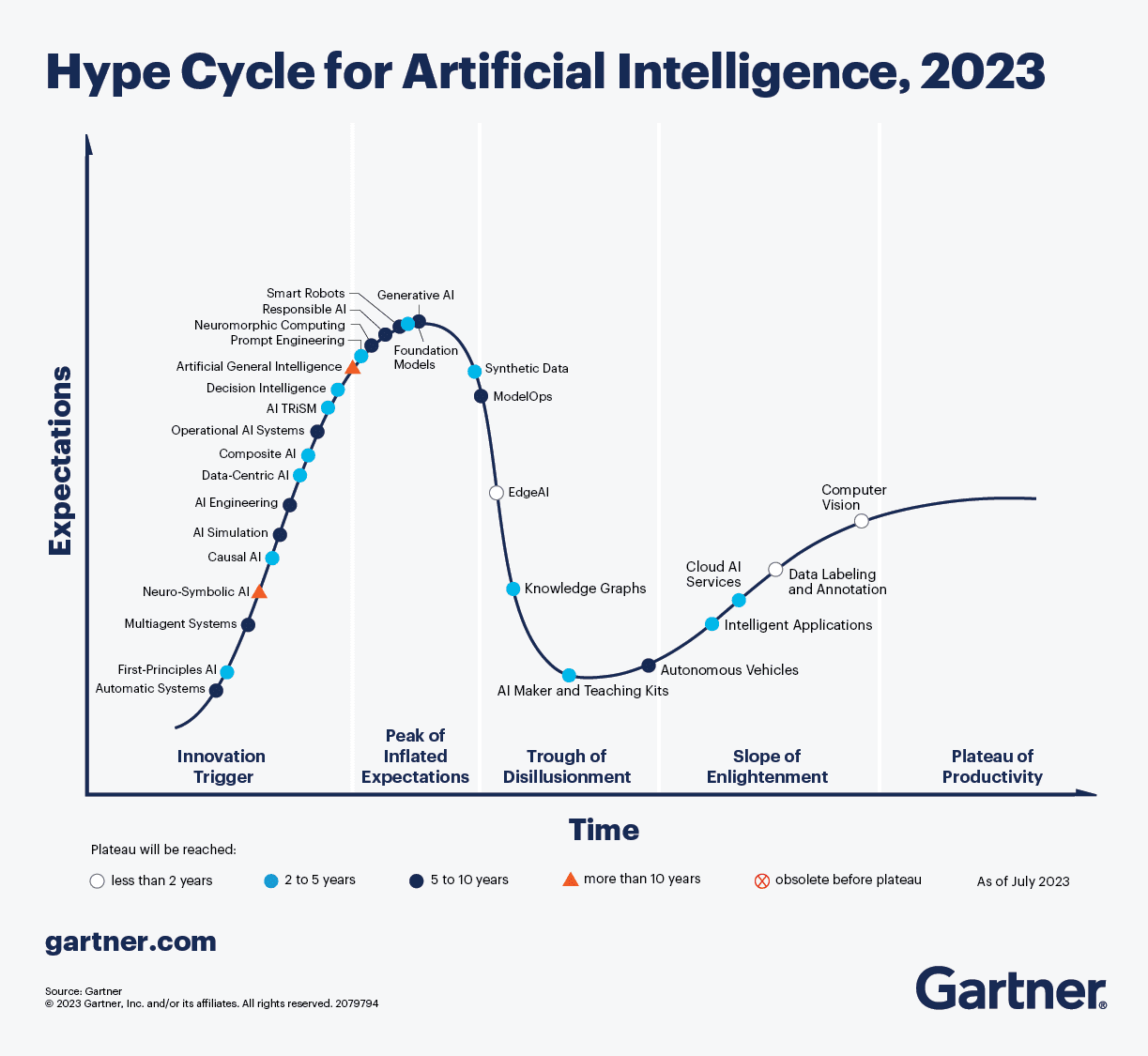
Gartner Hype Cycle for AI in 2023

Gartner Hype Cycle for AI in 2023
Image by Author

We all want to know what’s going on with technology. What’s new, what’s about to happen, what should I be learning, what companies are looking into?

You can learn all this with the 2023 Gartner Hype Cycle for Artificial Intelligence. The Gartner Hype Cycle provides you with graphic representations of technologies and applications, and what this means for real business problems and future opportunities.

The 2023 Gartner Hype Cycle™ for Artificial Intelligence (AI) identifies innovations and techniques that are currently providing us with significant benefits while also taking into consideration the risks that come with it.

Many of you have probably been wondering what will happen with technology now, especially since the rise of large language models (LLMs) such as ChatGPT. GenerativeAI is taking over, and we all want to know more! So what has the Gartner Hype Cycle informed us?

To start, Gartner suggests that there are two sides of Generative AI:

  • Innovations that will be fueled by Generative AI
  • Innovations that will fuel advances in Generative AI

Innovation Fueled by Generative AI

Generative AI will change a lot of things, and some of the areas that it will fuel innovation in are:

  • Artificial General Intelligence
  • AI Engineering
  • Autonomic Systems
  • Cloud AI Services
  • Composite AI
  • Computer Vision
  • Data-centric AI
  • Edge AI
  • Intelligent Applications
  • Model Operationalization
  • Operational AI Systems
  • Prompt Engineering
  • Smart Robots
  • Synthetic data

Innovation Fueling Advances in Generative AI

So what are the areas that will fuel advances in Generative AI? They are:

  • AI Simulation
  • AI trust, risk and security management (AI TRiSM)
  • Causal AI
  • Data Labeling and Annotation
  • First-principles AI (FPAI)
  • Foundation Models
  • Knowledge Graphs
  • Multiagent Systems (MAS)
  • Neurosymbolic AI
  • Responsible AI

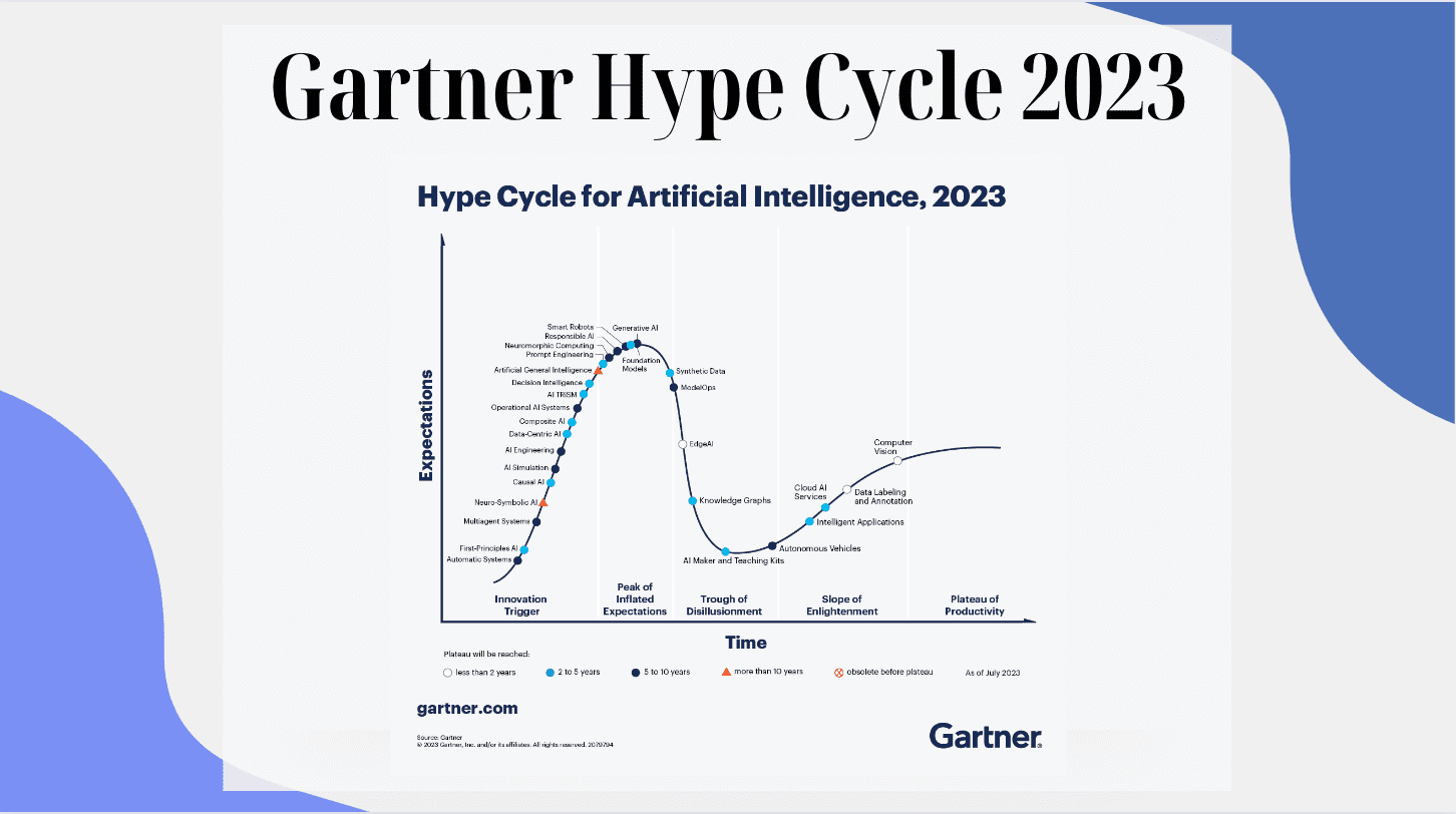
Want to know how long it will take for these innovations to trigger and plateau. Have a deeper look into the Gartner Hype Cycle visualization below:

Gartner Hype Cycle for AI in 2023
Image by Gartner Hype Cycle Wrapping it up

Gartner has provided us with a new way to look at what Generative AI can do for us and how it is going to shape our future. The visualizations give us an estimated time frame on what to expect in the future. Based on what you’ve learned in this article, would you challenge anything? Let us know in the comments.
Nisha Arya is a Data Scientist, Freelance Technical Writer and Community Manager at KDnuggets. She is particularly interested in providing Data Science career advice or tutorials and theory based knowledge around Data Science. She also wishes to explore the different ways Artificial Intelligence is/can benefit the longevity of human life. A keen learner, seeking to broaden her tech knowledge and writing skills, whilst helping guide others.

More On This Topic

  • Unlock DataOps Success with DataOps.live — Featured in Gartner Market…
  • Unlock DataOps Success with DataOps.live: Featured in Gartner Market Guide!
  • 10 Amazing Machine Learning Visualizations You Should Know in 2023
  • Top Data Python Packages to Know in 2023
  • Google Data Analytics Certification Review for 2023
  • 5 Free Data Science Books You Must Read in 2023

Tesla Optimus Finally Learns Yoga, Performs Vrikshasana

Optimus Finally Learns Yoga Moves, Performs Vrikshasana

Almost a year ago, Elon Musk unveiled prototype ofTesla’s Humanoid robot Optimus. It was still in the early stages of development, not much was revealed by the company how exactly it functioned. Now, Tesla has announced major improvements in its Humanoid robots, and it looks like it is moving closer to what Musk has envisioned with Optimus.

pic.twitter.com/30mCr2Duk9

— Elon Musk (@elonmusk) September 25, 2023

Last year, Optimus just waved on the stage. Now, it can pick up and sort objects, do yoga, and navigate through surroundings. Moreover, compared to others such as Boston Dynamics, it has its fingers working and working on neural networks, not just rules. All of this within just two years.

Reverse engineering Optimus’ motion

Last year, during the unveiling of Optimus, looking at the bipedal movement, it might be balancing its movement using the technique called Zero-Moment Point. That might still be true, but the humanoid has definitely made a lot of improvements.

Jim Fan, Senior AI scientist at NVIDIA, did an in depth analysis and has given a lot of insights about how exactly Optimus works and functions with such brilliance.

The impressive smooth hand movements, owes its dexterity to a unique approach to learning. It’s highly likely that these fluid motions have been cultivated through a process known as imitation learning, often referred to as “behaviour cloning.” Essentially, this means the robot learns by mimicking human operators. This is similar to how animations are recorded for characters within games.

The alternative method, which involves reinforcement learning in a simulated environment, typically results in jerky movements and unnatural hand poses.

Motion Capture (MoCap): Some of Optimus’s hand movements might be recorded using motion capture technology, similar to what’s used in Hollywood movies. By wearing a device like the CyberGlove, a demonstrator can capture real-time hand motion signals and haptic feedback, which can then be applied to Optimus.

Custom Control System: This method likely involves a specially designed teleoperation system, allowing human operators to precisely control the robot’s movements. A noteworthy example of this approach is ALOHA, developed by Stanford AI Labs. ALOHA enables intricate, dexterous motions, such as handling tiny objects like AAA batteries or manipulating contact lenses.

Computer Vision MoCap: In contrast to wearing markers or gloves, Optimus might use computer vision for motion capture. Technologies like DexPilot from NVIDIA enable marker-less and glove-free data collection. Human operators can simply use their bare hands to perform tasks while cameras and GPUs translate their motions into data for robot learning.

VR Headset: Another intriguing method involves turning the training process into a virtual reality game. Operators can “role play” as Optimus using VR controllers or CyberGloves. This approach offers the advantage of scalability, as annotators from around the world can contribute without needing to be physically present.

It’s worth noting that Optimus could employ a combination of these methods, each with its own set of advantages and disadvantages.

Neural Architecture of Optimus

Optimus’s ability to learn from human demonstrations and exhibit precise hand movements is facilitated by a sophisticated neural architecture. The robot is trained in an end-to-end manner, which means it takes in videos as input and produces actions as output.

Image Processing: Optimus analyses images to understand its surroundings. This could involve using efficient Vision Transformers (ViT) or more conventional backbone models like ResNet or EfficientNet.

Video Analysis: Videos can be processed in two ways—treating each frame as an individual image or considering the video as a whole. Different techniques, such as SlowFast Network or RubiksNet, are used to efficiently handle video data.

Language Integration: While it’s not entirely clear whether Optimus responds to language prompts, if it does, there’s a mechanism for integrating language with visual perception. Techniques like Feature-wise Linear Modulation (FiLM) may be employed for this purpose, allowing language embeddings to influence the image processing pathway.

Action Tokenisation: To translate continuous motion signals into discrete actions that the robot can understand, Optimus might use various methods, such as categorising the movements or employing VQVAE for compression.

All these components work together within a Transformer-based controller. This controller takes in video tokens (possibly modulated by language) and produces action tokens step by step. The robot continually refines its actions by observing the consequences of its previous moves, demonstrating its self-corrective abilities as seen in the demos.

How many Optimus does the world need?

Musk confidently said that everyone in the future would want to have one Optimus for themselves. Or it might be even more than one.

Expect Optimus.pic.twitter.com/btE0gnjnWf

— Smoke-away (@SmokeAwayyy) September 24, 2023

Tesla has moved away from being just a car company, and is completely an AI company now. It is hiring for various AI roles, specifically for building Optimus. Moreover, several companies such as RoboFab, Figure.ai, Boston Dynamics, Chinese company Fourier Intelligence, and even OpenAI’s investment in 1X robotics company, hints that the next year would be for humanoid robots.

Coexistence of humans and robots might arrive sooner than we think. And the future will never be the same.

The post Tesla Optimus Finally Learns Yoga, Performs Vrikshasana appeared first on Analytics India Magazine.