Time series analysis is widely used for forecasting and predicting future points in a time series. AutoRegressive Integrated Moving Average (ARIMA) models are widely used for time series forecasting and are considered one of the most popular approaches. In this tutorial, we will learn how to build and evaluate ARIMA models for time series forecasting in Python.
What is an ARIMA Model?
The ARIMA model is a statistical model utilized for analyzing and predicting time series data. The ARIMA approach explicitly caters to standard structures found in time series, providing a simple yet powerful method for making skillful time series forecasts.
ARIMA stands for AutoRegressive Integrated Moving Average. It combines three key aspects:
- Autoregression (AR): A model that uses the correlation between the current observation and lagged observations. The number of lagged observations is referred to as the lag order or p.
- Integrated (I): The use of differencing of raw observations to make the time series stationary. The number of differencing operations is referred to as d.
- Moving Average (MA): A model takes into account the relationship between the current observation and the residual errors from a moving average model applied to past observations. The size of the moving average window is the order or q.
The ARIMA model is defined with the notation ARIMA(p,d,q) where p, d, and q are substituted with integer values to specify the exact model being used.
Key assumptions when adopting an ARIMA model:
- The time series was generated from an underlying ARIMA process.
- The parameters p, d, q must be appropriately specified based on the raw observations.
- The time series data must be made stationary via differencing before fitting the ARIMA model.
- The residuals should be uncorrelated and normally distributed if the model fits well.
In summary, the ARIMA model provides a structured and configurable approach for modeling time series data for purposes like forecasting. Next we will look at fitting ARIMA models in Python.
Python Code Example
In this tutorial, we will use Netflix Stock Data from Kaggle to forecast the Netflix stock price using the ARIMA model.
Data Loading
We will load our stock price dataset with the “Date” column as index.
import pandas as pd net_df = pd.read_csv("Netflix_stock_history.csv", index_col="Date", parse_dates=True) net_df.head(3) 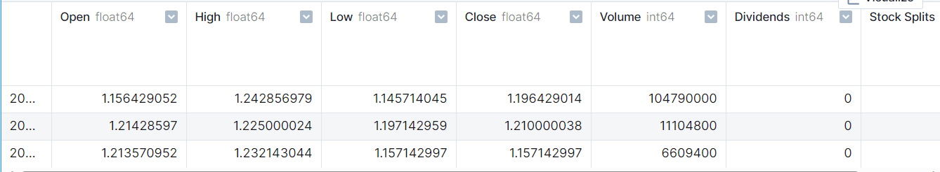
Data Visualization
We can use pandas 'plot' function to visualize the changes in stock price and volume over time. It's clear that the stock prices are increasing exponentially.
net_df[["Close","Volume"]].plot(subplots=True, layout=(2,1)); 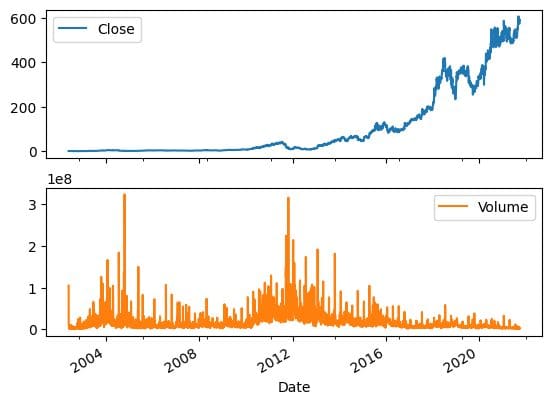
Rolling Forecast ARIMA Model
Our dataset has been split into training and test sets, and we proceeded to train an ARIMA model. The first prediction was then forecasted.
We received a poor outcome with the generic ARIMA model, as it produced a flat line. Therefore, we have decided to try a rolling forecast method.
Note: The code example is a modified version of the notebook by BOGDAN IVANYUK.
from statsmodels.tsa.arima.model import ARIMA from sklearn.metrics import mean_squared_error, mean_absolute_error import math train_data, test_data = net_df[0:int(len(net_df)*0.9)], net_df[int(len(net_df)*0.9):] train_arima = train_data['Open'] test_arima = test_data['Open'] history = [x for x in train_arima] y = test_arima # make first prediction predictions = list() model = ARIMA(history, order=(1,1,0)) model_fit = model.fit() yhat = model_fit.forecast()[0] predictions.append(yhat) history.append(y[0])When dealing with time series data, a rolling forecast is often necessary due to the dependence on prior observations. One way to do this is to re-create the model after each new observation is received.
To keep track of all observations, we can manually maintain a list called history, which initially contains training data and to which new observations are appended each iteration. This approach can help us get an accurate forecasting model.
# rolling forecasts for i in range(1, len(y)): # predict model = ARIMA(history, order=(1,1,0)) model_fit = model.fit() yhat = model_fit.forecast()[0] # invert transformed prediction predictions.append(yhat) # observation obs = y[i] history.append(obs) Model Evaluation
Our rolling forecast ARIMA model showed a 100% improvement over simple implementation, yielding impressive results.
# report performance mse = mean_squared_error(y, predictions) print('MSE: '+str(mse)) mae = mean_absolute_error(y, predictions) print('MAE: '+str(mae)) rmse = math.sqrt(mean_squared_error(y, predictions)) print('RMSE: '+str(rmse))MSE: 116.89611817706545 MAE: 7.690948135967959 RMSE: 10.811850821069696Let's visualize and compare the actual results to the predicted ones . It's clear that our model has made highly accurate predictions.
import matplotlib.pyplot as plt plt.figure(figsize=(16,8)) plt.plot(net_df.index[-600:], net_df['Open'].tail(600), color='green', label = 'Train Stock Price') plt.plot(test_data.index, y, color = 'red', label = 'Real Stock Price') plt.plot(test_data.index, predictions, color = 'blue', label = 'Predicted Stock Price') plt.title('Netflix Stock Price Prediction') plt.xlabel('Time') plt.ylabel('Netflix Stock Price') plt.legend() plt.grid(True) plt.savefig('arima_model.pdf') plt.show() 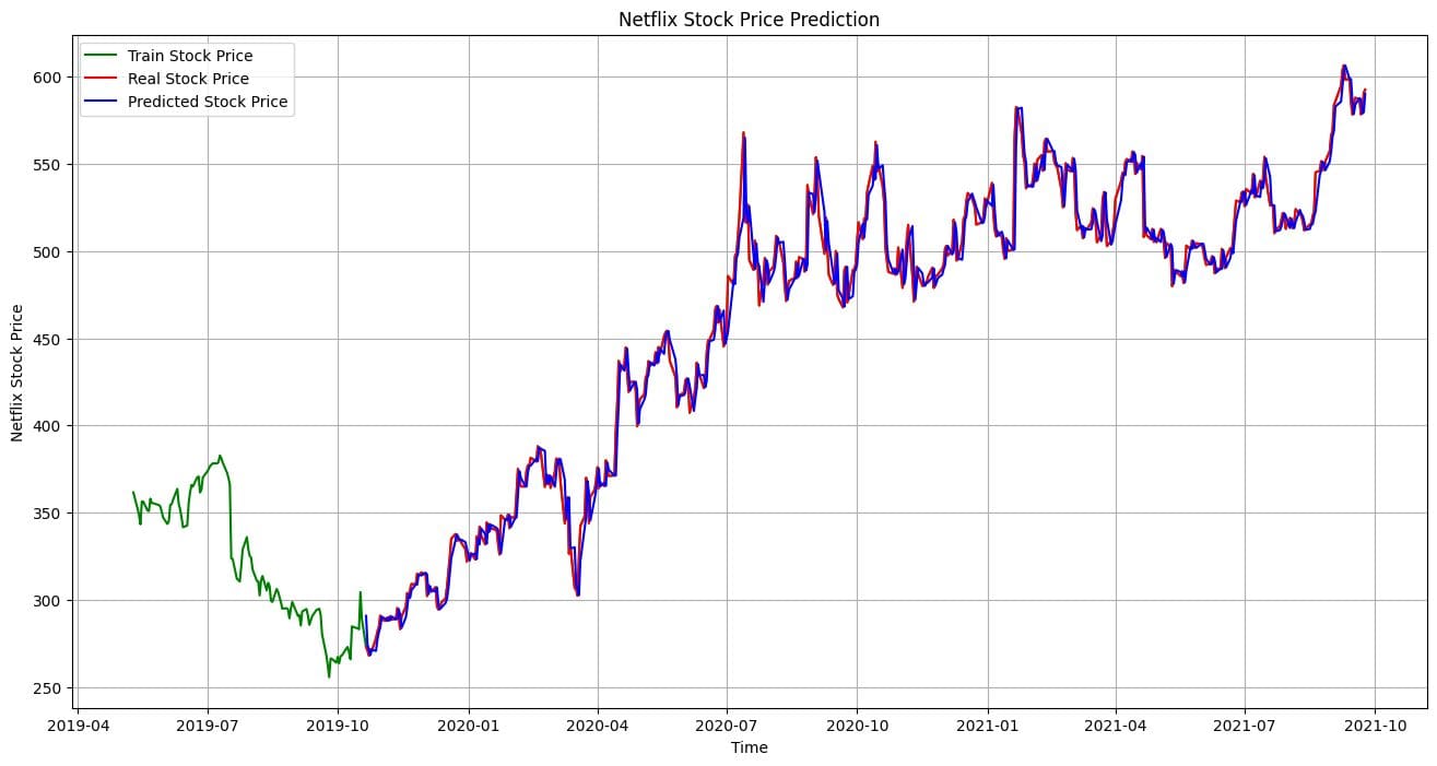 Conclusion
In this short tutorial, we provided an overview of ARIMA models and how to implement them in Python for time series forecasting. The ARIMA approach provides a flexible and structured way to model time series data that relies on prior observations as well as past prediction errors. If you're interested in a comprehensive analysis of the ARIMA model and Time Series analysis, I recommend taking a look at Stock Market Forecasting Using Time Series Analysis.
Abid Ali Awan (@1abidaliawan) is a certified data scientist professional who loves building machine learning models. Currently, he is focusing on content creation and writing technical blogs on machine learning and data science technologies. Abid holds a Master's degree in Technology Management and a bachelor's degree in Telecommunication Engineering. His vision is to build an AI product using a graph neural network for students struggling with mental illness.
- Time Series Forecasting with Ploomber, Arima, Python, and Slurm
- Codeless Time Series Analysis with KNIME
- Full cross-validation and generating learning curves for time-series models
- Multivariate Time Series Analysis with an LSTM based RNN
- Market Data and News: A Time Series Analysis
- Create a Time Series Ratio Analysis Dashboard