Streamline Your Machine Learning Workflow with Scikit-learn Pipelines

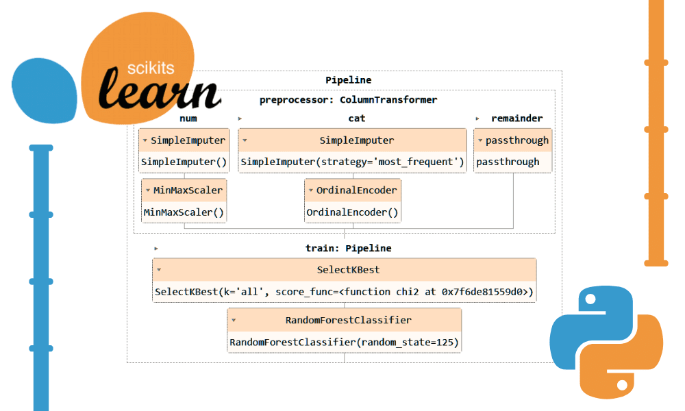
Image by Author

Using Scikit-learn pipelines can simplify your preprocessing and modeling steps, reduce code complexity, ensure consistency in data preprocessing, help with hyperparameter tuning, and make your workflow more organized and easier to maintain. By integrating multiple transformations and the final model into a single entity, Pipelines enhance reproducibility and make everything more efficient.

In this tutorial, we will be working with the Bank Churn dataset from Kaggle to train a Random Forest Classifier. We will compare the conventional approach of data preprocessing and model training with a more efficient method using Scikit-learn pipelines and ColumnTransformers.

Data Processing Pipeline

In the data processing pipeline, we will learn how to transform both categorical and numerical columns individually. We will start with a traditional style of code and then show a better way to perform similar processing.

After extracting the data from the zip file, load the `train.csv` file with “id” as the index column. Drop unnecessary columns and shuffle the dataset.

import pandas as pd    bank_df = pd.read_csv("train.csv", index_col="id")  bank_df = bank_df.drop(['CustomerId', 'Surname'], axis=1)  bank_df = bank_df.sample(frac=1)  bank_df.head()

We have categorical, integer, and float columns. The dataset looks pretty clean.

Simple Scikit-learn Code

As a data scientist, I have written this code multiple times. Our objective is to fill in the missing values for both categorical and numerical features. To achieve this, we will use a `SimpleImputer` with different strategies for each type of feature.

After the missing values are filled in, we will convert categorical features to integers and apply min-max scaling on numerical features.

from sklearn.impute import SimpleImputer  from sklearn.preprocessing import OrdinalEncoder, MinMaxScaler    cat_col = [1,2]  num_col = [0,3,4,5,6,7,8,9]    # Filling missing categorical values  cat_impute = SimpleImputer(strategy="most_frequent")  bank_df.iloc[:,cat_col] = cat_impute.fit_transform(bank_df.iloc[:,cat_col])    # Filling missing numerical values  num_impute = SimpleImputer(strategy="median")  bank_df.iloc[:,num_col] = num_impute.fit_transform(bank_df.iloc[:,num_col])      # Encode categorical features as an integer array.  cat_encode = OrdinalEncoder()  bank_df.iloc[:,cat_col] = cat_encode.fit_transform(bank_df.iloc[:,cat_col])      # Scaling numerical values.  scaler = MinMaxScaler()  bank_df.iloc[:,num_col] = scaler.fit_transform(bank_df.iloc[:,num_col])    bank_df.head()

As a result, we got a dataset that is clean and transformed with only integer or float values.

Scikit-learn Pipelines Code

Let’s convert the above code using the `Pipeline` and `ColumnTransformer`. Instead of applying the preprocessing technique, we will create two pipelines. One is for numerical columns, and one is for categorical columns.

1. In the numerical pipeline, we have used a simple impute with a “mean” strategy and applied a min-max scaler for normalization.
2. In the categorical pipeline, we used the simple imputer with the “most_frequent“ strategy and the original encoder to convert the categories into numerical values.

We combined the two pipelines using the ColumnTransformer and provided each with the columns index. It will help you apply these pipelines on certain columns. For example, a categorical transformer pipeline will be applied to only columns 1 and 2.

Note: the remainder="passthrough" means that the columns that have not been processed will be added in the end. In our case, it is the target column.

from sklearn.impute import SimpleImputer  from sklearn.preprocessing import OrdinalEncoder, MinMaxScaler  from sklearn.compose import ColumnTransformer  from sklearn.pipeline import Pipeline      # Identify numerical and categorical columns  cat_col = [1,2]  num_col = [0,3,4,5,6,7,8,9]    # Transformers for numerical data  numerical_transformer = Pipeline(steps=[      ('imputer', SimpleImputer(strategy='mean')),      ('scaler', MinMaxScaler())  ])    # Transformers for categorical data  categorical_transformer = Pipeline(steps=[      ('imputer', SimpleImputer(strategy='most_frequent')),      ('encoder', OrdinalEncoder())  ])    # Combine transformers into a ColumnTransformer  preproc_pipe = ColumnTransformer(      transformers=[          ('num', numerical_transformer, num_col),          ('cat', categorical_transformer, cat_col)      ],      remainder="passthrough"  )    # Apply the preprocessing pipeline  bank_df = preproc_pipe.fit_transform(bank_df)  bank_df[0]

After the transformation, the resulting array contains numerical transform value at the start and categorical transform value at the end, based on the order of the pipelines in the column transformer.

array([0.712     , 0.24324324, 0.6       , 0.        , 0.33333333,         1.        , 1.        , 0.76443485, 2.        , 0.        ,         0.        ])

You can run the pipeline object in the Jupyter Notebook to visualize the pipeline. Make sure you have the latest version of Scikit-learn.

preproc_pipe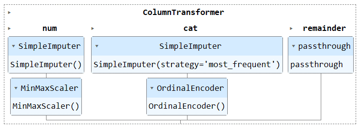

Data Training Pipeline

To train and evaluate our model, we need to split our dataset into two subsets: training and testing.

To do this, we will first create dependent and independent variables and convert them into NumPy arrays. Then, we will use the `train_test_split` function to split the dataset into two subsets.

from sklearn.model_selection import train_test_split    X = bank_df.drop("Exited", axis=1).values  y = bank_df.Exited.values    X_train, X_test, y_train, y_test = train_test_split(      X, y, test_size=0.3, random_state=125  )

Simple Scikit-learn Code

The conventional way of writing training code is to first perform feature selection using `SelectKBest` and then provide the new feature to our Random Forest Classifier model.

We will first train the model using the training set and evaluate the results using the testing dataset.

from sklearn.feature_selection import SelectKBest, chi2  from sklearn.ensemble import RandomForestClassifier    KBest = SelectKBest(chi2, k="all")  X_train = KBest.fit_transform(X_train, y_train)  X_test = KBest.transform(X_test)    model = RandomForestClassifier(n_estimators=100, random_state=125)    model.fit(X_train,y_train)    model.score(X_test, y_test)

We achieved a reasonably good accuracy score.

0.8613035487063481

Scikit-learn Pipelines Code

Let's use the `Pipeline` function to combine both training steps into a pipeline. We can then fit the model on the training set and evaluate it on the testing set.

KBest = SelectKBest(chi2, k="all")  model = RandomForestClassifier(n_estimators=100, random_state=125)    train_pipe = Pipeline(      steps=[          ("KBest", KBest),          ("RFmodel", model),      ]  )    train_pipe.fit(X_train,y_train)    train_pipe.score(X_test, y_test)

We achieved similar results, but the code appears to be more efficient and straightforward. It's quite easy to add or remove new steps from the training pipeline.

0.8613035487063481

Run the pipeline object to visualize the pipeline.

train_pipe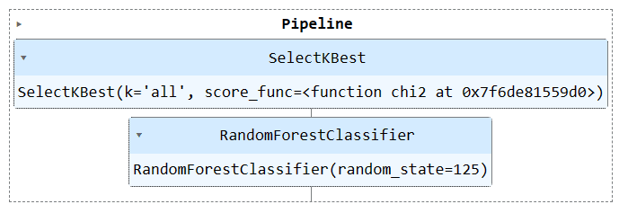

Combining Processing & Training Pipelines

Now, we will combine both preprocessing and training pipeline by creating another pipeline and adding both pipelines.

Here is the complete code:

import pandas as pd  from sklearn.model_selection import train_test_split  from sklearn.impute import SimpleImputer  from sklearn.preprocessing import OrdinalEncoder, MinMaxScaler  from sklearn.compose import ColumnTransformer  from sklearn.pipeline import Pipeline  from sklearn.feature_selection import SelectKBest, chi2  from sklearn.ensemble import RandomForestClassifier    #loading the data  bank_df = pd.read_csv("train.csv", index_col="id")  bank_df = bank_df.drop(['CustomerId', 'Surname'], axis=1)  bank_df = bank_df.sample(frac=1)      # Splitting data into training and testing sets  X = bank_df.drop(["Exited"],axis=1)  y = bank_df.Exited    X_train, X_test, y_train, y_test = train_test_split(      X, y, test_size=0.3, random_state=125  )    # Identify numerical and categorical columns  cat_col = [1,2]  num_col = [0,3,4,5,6,7,8,9]    # Transformers for numerical data  numerical_transformer = Pipeline(steps=[      ('imputer', SimpleImputer(strategy='mean')),      ('scaler', MinMaxScaler())  ])    # Transformers for categorical data  categorical_transformer = Pipeline(steps=[      ('imputer', SimpleImputer(strategy='most_frequent')),      ('encoder', OrdinalEncoder())  ])    # Combine pipelines using ColumnTransformer  preproc_pipe = ColumnTransformer(      transformers=[          ('num', numerical_transformer, num_col),          ('cat', categorical_transformer, cat_col)      ],      remainder="passthrough"  )    # Selecting the best features  KBest = SelectKBest(chi2, k="all")    # Random Forest Classifier  model = RandomForestClassifier(n_estimators=100, random_state=125)    # KBest and model pipeline  train_pipe = Pipeline(      steps=[          ("KBest", KBest),          ("RFmodel", model),      ]  )    # Combining the preprocessing and training pipelines  complete_pipe = Pipeline(      steps=[                   ("preprocessor", preproc_pipe),          ("train", train_pipe),      ]  )    # running the complete pipeline  complete_pipe.fit(X_train,y_train)    # model accuracy  complete_pipe.score(X_test, y_test)

Output:

0.8592837955201874

Visualizing the complete pipeline.

complete_pipe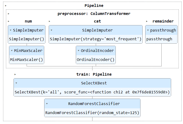

Saving and Loading the Model

One of the major advantages of using pipelines is that you can save the pipeline with the model. During inference, you only need to load the pipeline object, which will be ready to process the raw data and provide you with accurate predictions. You don't need to re-write the processing and transformation functions in the app file, as it will work out of the box. This makes the machine learning workflow more efficient and saves time.

Let’s first save the pipeline using the skops-dev/skops library.

import skops.io as sio    sio.dump(complete_pipe, "bank_pipeline.skops")

Then, load the saved pipeline and display the pipeline.

new_pipe = sio.load("bank_pipeline.skops", trusted=True)  new_pipe

As we can see, we have successfully loaded the pipeline.

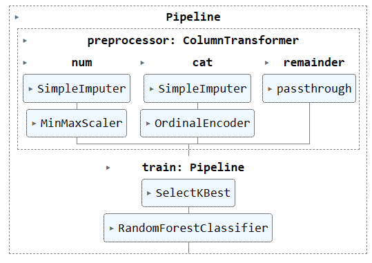
To evaluate our loaded pipeline, we will make predictions on the test set and then calculate accuracy and F1 scores.

from sklearn.metrics import accuracy_score, f1_score    predictions = new_pipe.predict(X_test)  accuracy = accuracy_score(y_test, predictions)  f1 = f1_score(y_test, predictions, average="macro")    print("Accuracy:", str(round(accuracy, 2) * 100) + "%", "F1:", round(f1, 2))

It turns out we need to focus on minority classes to improve our f1 score.

Accuracy: 86.0% F1: 0.76

The project files and code is available on Deepnote Workspace. The workspace has two Notebooks: One with the Scikit-learn pipeline and one without it.

Conclusion

In this tutorial, we learned how Scikit-learn pipelines can help streamline machine learning workflows by chaining together sequences of data transforms and models. By combining preprocessing and model training into a single Pipeline object, we can simplify code, ensure consistent data transformations, and make our workflows more organized and reproducible.

Abid Ali Awan (@1abidaliawan) is a certified data scientist professional who loves building machine learning models. Currently, he is focusing on content creation and writing technical blogs on machine learning and data science technologies. Abid holds a Master's degree in Technology Management and a bachelor's degree in Telecommunication Engineering. His vision is to build an AI product using a graph neural network for students struggling with mental illness.

More On This Topic

• Easily Integrate LLMs into Your Scikit-learn Workflow with Scikit-LLM
• Beyond Pipelines: Graphs as Scikit-Learn Metaestimators
• RAPIDS cuDF to Speed up Your Next Data Science Workflow
• Visualizing Your Confusion Matrix in Scikit-learn
• Getting Started with Scikit-learn for Classification in Machine Learning
• Scikit-learn for Machine Learning Cheat Sheet