OpenAI brings the competition to DeepMind’s doorstep with new London office

OpenAI brings the competition to DeepMind’s doorstep with new London office Kyle Wiggers 7 hours

OpenAI is expanding overseas. To London, specifically.

Today, the Microsoft-backed AI startup announced that it plans to open an office in London, its first international outpost. When OpenAI’s London location opens its doors, it’ll focus on advancing “research and engineering capabilities” while balancing collaborating with “local communities and policymakers,” according to CEO Sam Altman.

“We see this expansion as an opportunity to attract world-class talent and drive innovation in AGI development and policy,” Altman, who reportedly had floated Poland and France as alternatives for the office, said in a canned statement. “We’re excited about what the future holds and to see the contributions our London office will make towards building and deploying safe AI.”

London is a conspicuous choice for OpenAI, which hasn’t expanded beyond its San Francisco headquarters since its founding in 2015. The city is the longtime home base of DeepMind, Google’s largest AI research division, and a wellspring of data science talent, owing to its rich academic history and renowned universities.

Broadly speaking, London is also becoming a booming center for AI startup ventures. According to a recent report, as of 2021, over 1,300 AI companies were based in London and the city was the top-funded in the U.K. in terms of venture dollars invested.

The city is also important politically to tech companies heavily invested in AI, like OpenAI, who seek to convince the U.K.’s governing bodies to regulate AI with a light touch. On a recent lobbying tour, Altman made an appearance at the University College London, where he called for “balanced” regulation and warned of the risks of deepfake disinformation.

At that same appearance, Altman said that OpenAI would “cease operating” in the European Union if it’s unable to comply with the provisions of the bloc’s AI Act, one of the first comprehensive set of regulations for the AI industry. He later backed down from the comments — but the play was made.

OpenAI Expands to London

OpenAI Updates

After Sam Altman completes his world tour in search of expanding its office and talking about AI all over the world, OpenAI today announced that it has decided to open an office in London. This is the first corporate office outside the US.

OpenAI announced in a blog post its intention to hire individuals for research, engineering, and business roles in London, a city that Altman praised for its exceptional talent pool. It is worth noting that DeepMind, a research lab that spearheads AI strategy for Alphabet Inc.’s Google and serves as one of OpenAI’s main competitors, is also situated in London.

Altman, while expressing OpenAI’s vision towards building AGI, said, “we see this expansion as an opportunity to attract world-class talent and drive innovation in AGI development and policy.”

The company based in San Francisco has been actively recruiting new employees in order to monetize its expensive AI research. Altman has expressed interest in opening a European office, considering countries like Poland, France, and the UK as potential options. This decision comes at a time when the UK and France are competing to establish themselves as the leading tech hub in Europe. Mistral AI, a startup coming up to compete with OpenAI, is also based in Europe in Paris.

During his visit to London, Altman had a meeting with UK Prime Minister Rishi Sunak. He also criticised the European Union’s approach to regulating AI, initially suggesting that OpenAI might stop operating in the region if they were unable to comply with upcoming regulations, although he later retracted his statement.

In recent news, Altman had also shown interest in building its own marketplace for AI models that are built on its technology. Moreover, the company has also announced that it is integrating ChatGPT’s iOS app with Bing.

The post OpenAI Expands to London appeared first on Analytics India Magazine.

Google Launches ONDC Accelerator Program to Revolutionise E-commerce in India

Google recently held its first I/O Connect event in India, where it unveiled a range of AI tools and technologies aimed at supporting growth and innovation among local developers. The announcements made during the event emphasised Google’s commitment to helping developers build AI-powered products in a productive, creative, and responsible manner.

One of the key initiatives introduced by Google Cloud is an accelerator program for the Open Network for Digital Commerce (ONDC). This program aims to assist India’s digital sellers in building and scaling their digital commerce operations. As part of this effort, Google Cloud is open-sourcing a ready implementation of the ONDC infrastructure and core APIs to facilitate scalability and security. Additionally, Google Cloud is providing access to its Retail AI technology and PaLM API. Furthermore, a startup credits program has been introduced, allowing organisations enabling ONDC to apply for a grant of USD $25,000.

Another significant announcement made by Google is the open-sourcing of its research models and datasets, specifically focused on India. This initiative aims to help developers create meaningful solutions using India-focused speech data and building information.

T Koshy, the Managing Director and CEO at ONDC, expressed enthusiasm about Google Cloud’s Accelerator Program, stating that it reinforces ONDC’s mission to revolutionise the e-commerce landscape and bring about increased efficiency, agility, and customer-centricity. By simplifying the onboarding process through efficient core APIs, this addition to the open network empowers enterprises to focus on their core competencies.

“The addition of Google Cloud’s Accelerator Program reinforces ONDC’s mission to revolutionise the ecommerce landscape, ushering in a new era of efficiency, agility, and customer-centricity. By streamlining the onboarding process through efficient core APIs, this milestone addition to the open network empowers enterprises to focus on their core competencies,” koshy said.

In recent times, ONDC has been working to streamline its onboarding process and enhance its payments and settlements. One such effort involves a collaboration between Protean and NPCI Bharat BillPay Limited. They have launched the Recon & Settlement Product (RSP) on the NBBL’s NOCS platform, serving as a Settlement Agency (SA) to enhance ONDC’s payments and settlements. Additionally, Shiprocket‘s Seller App has been introduced to streamline ONDC onboarding and integration for merchants, addressing previous concerns about the onboarding process being slower compared to platforms like UPI, as acknowledged by ONDC’s CTO, Nitin Mishra in a conversation with AIM.

The post Google Launches ONDC Accelerator Program to Revolutionise E-commerce in India appeared first on Analytics India Magazine.

Slang taps AI to answer phone calls for brick-and-mortar businesses

Slang taps AI to answer phone calls for brick-and-mortar businesses Kyle Wiggers 8 hours

For business owners, phone calls can be an enormous time waster. Take the restaurant industry, for example. Calls can lead to more important tasks being overlooked, like doing inventory, balancing staff schedules, running payroll and fixing equipment issues. The issue, exacerbated by the pandemic, is so severe that restaurants are increasingly abandoning their phone lines.

Alex Sambvani and Gabriel Duncan, who met while working at Spotify, set out to solve the problem of overwhelming incoming calls using AI, drawing on their backgrounds as data scientists. What emerged from their joint work is Slang.ai, a platform that automatically answers the phone for restaurants, retailers and other types of brick-and-mortar businesses.

“Slang acts like a reliable team member that gives accurate responses and helps drive more revenue, giving businesses AI superpowers and empowering them to provide exceptional service to callers and streamline operations in a personalized manner,” Sambvani told TechCrunch via email.

In plainer, less jargony and fluffy English, Slang acts as a sort of digital phone concierge that answers questions and takes — or modifies — reservations, including OpenTable and Resy reservations via integrations. Using Slang, callers can book or modify reservations or even simply let a business know that they’re running late.

Slang.ai

Image Credits: Slang.ai

Businesses can decide which calls Slang handles automatically versus hands off to staff. Sambvani claims that Slang’s automatic speech recognition works for callers of all ages and understands different accents — an impressive feat if true, given automatic speech recognition tech’s historically poor handling of diverse dialects.

“Many brick-and-mortar businesses are understaffed, causing them to miss calls and send potential customers to voicemail where they lose out on potential revenue,” he continued. “Slang provides its clients access to previously unknown data about why customers are calling … [And it] can surface trending reasons why customers are calling and can help operators proactively identify opportunities or issues, such as a location getting an abnormal amount of complaints relative to other locations.”

Slang isn’t the only startup selling a vision of tech to cut down on unnecessary phone interactions. There’s Goodcall, which offers a free cloud-based, AI-powered conversational platform to manage incoming phone calls. Kea is building phone-answering AI specifically for restaurants. So is ConverseNow, whose AI voice assistants take orders in quick service restaurants via the phone, chat, drive-thru and self-service kiosks.

So what does Slang bring to the table that sets it apart? A large customer base, mainly, According to Sambvani, Slang has over 200 clients today, including Slutty Vegan, Palm House Hospitality Group, Studs, Planta, Hammitt and Nikki Beach Miami. Revenue grew 6x in 2022.

Slang.ai

Image Credits: Slang.ai

That success led investors to pour $20 million into Slang — $8 million as a part of a seed round and $12 million in a Series A. Homebrew led the latter with participation from Stage 2 Capital, Wing VC, Underscore VC, Active Capital and Collide Capital.

Sambvani says that the proceeds will be used to establish new partnerships and integrations in the restaurant, hospitality, retail and ecommerce industries, grow Slang’s go-to-market team and expand headcount from 18 employees to 40 by the end of the year.

Fosfor and Snowflake Join Forces for Enhanced Enterprise Decision-making with Generative AI 

Top 7 Free Resources To Learn Snowflake

At Snowflake Summit 2023, Fosfor, a data products unit of LTIMindtree, recently announced a series of new integrations with Snowflake.

With this partnership, the dup looks to enable Snowflake customers to make the most of the data cloud. By integrating the Fosfor Decision Cloud, customers can speed up their use of artificial intelligence and machine learning tasks while enhancing their ability to make intelligent decisions on a large scale within their organizations, the company said in a statement.

The first integration will help the enterprises by combining capabilities of Fosfor’s decision intelligence product, Lumin Flow, powered by GPT, making it possible for Snowflake customers to get actionable insights quickly, safely, and securely, the company said.

“By bringing the power of GPT to Lumin, our vision is to democratize decision making on the data cloud,” said Debasis Satpathy, Chief Business Officer, Fosfor.

The second integration of Refract’s Streamlit with Lumin simplifies the creation of custom models for new applications.

Lumin provides a Streamlit SDK pack, combining the Snowflake tech stack with Lumin’s decision intelligence capabilities.

The third integration of Refract’s Snowpark with Lumin, which comes with natural language search capability and NLP-based insights, will enable customers to fully exploit the power of Snowpark and aid new use cases, which were not previously possible, the company said in the press release.

LTIMindtree launched Lumin earlier this year in March leveraging data analytics to identify trends, glean insights and make more effective, business-critical decisions. The company recently launched a generative AI platform called Canvas.ai.

The post Fosfor and Snowflake Join Forces for Enhanced Enterprise Decision-making with Generative AI appeared first on Analytics India Magazine.

Data Science Project of Rotten Tomatoes Movie Rating Prediction: First Approach

Data Science Project of Rotten Tomatoes Movie Rating Prediction: First ApproachImage by Author

It's no secret that predicting the success of a movie in the entertainment industry can make or break a studio's financial prospects.

Accurate predictions enable studios to make well-informed decisions about various aspects, such as marketing, distribution, and content creation.

Best of all, these predictions can help maximize profits and minimize losses by optimizing the allocation of resources.

Fortunately, machine learning techniques provide a powerful tool to tackle this complex problem. No doubt about it, by leveraging data-driven insights, studios can significantly improve their decision-making process.

This data science project has been used as a take-home assignment in the recruitment process at Meta (Facebook). In this take-home assignment, we will discover how Rotten Tomatoes is making labeling as ‘Rotten’, ‘Fresh’ or ‘Certified Fresh’.

To do that, we will develop two different approaches.
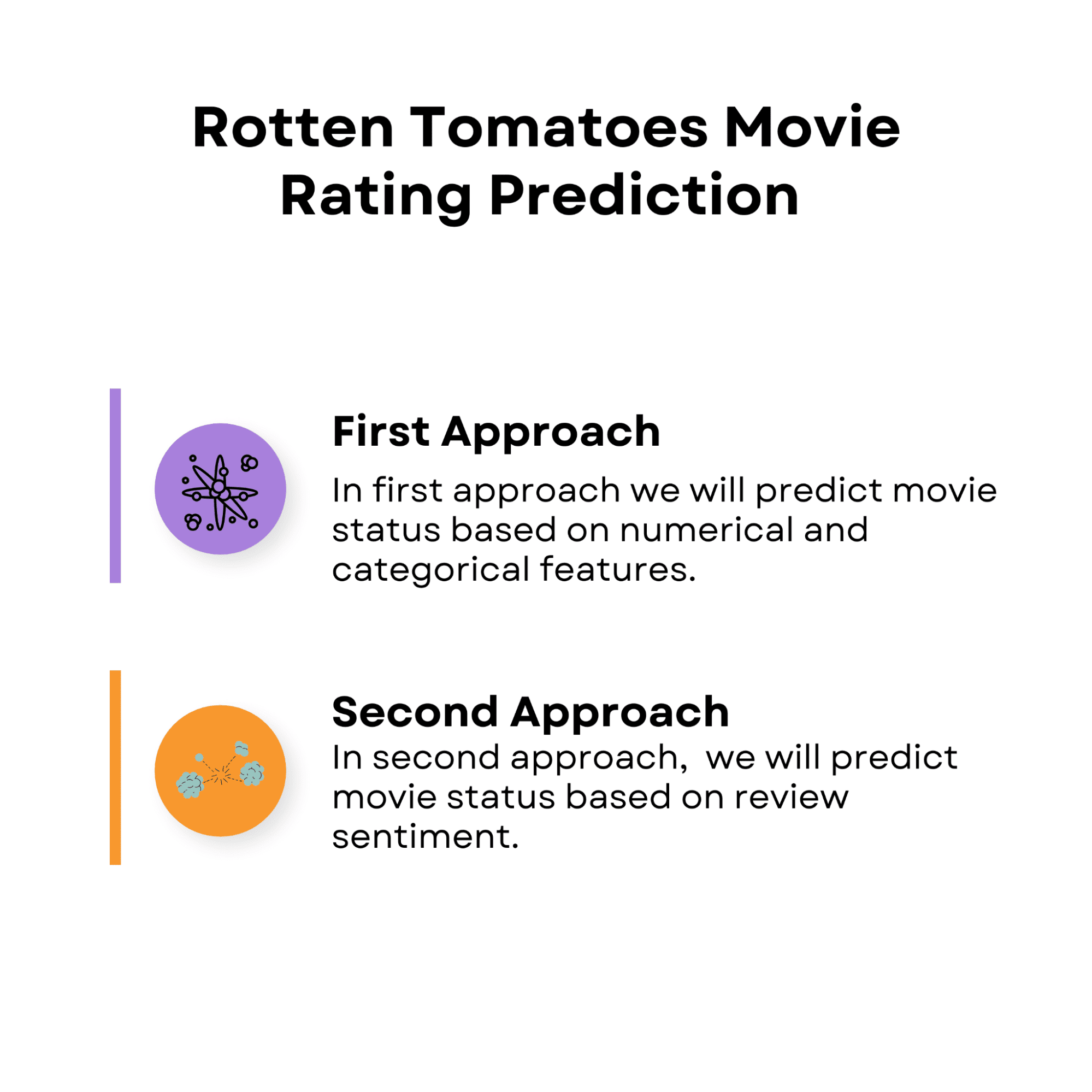
Data Science Project of Rotten Tomatoes Movie Rating Prediction: First Approach
Image by Author

Throughout our exploration, we will discuss data preprocessing, various classifiers, and potential improvements to enhance the performance of our models.

By the end of this post, you will have gained an understanding of how machine learning can be employed to predict movie success and how this knowledge can be applied in the entertainment industry.

But before going deeper, let’s discover the data we will work on.

First Approach: Predicting Movie Status Based on Numerical and Categorical Features

In this approach, we will use a combination of numerical and categorical features to predict the success of a movie.

The features we will consider include factors such as budget, genre, runtime, and director, among others.

We will employ several machine learning algorithms to build our models, including Decision Trees, Random Forests, and Weighted Random Forests with feature selection.
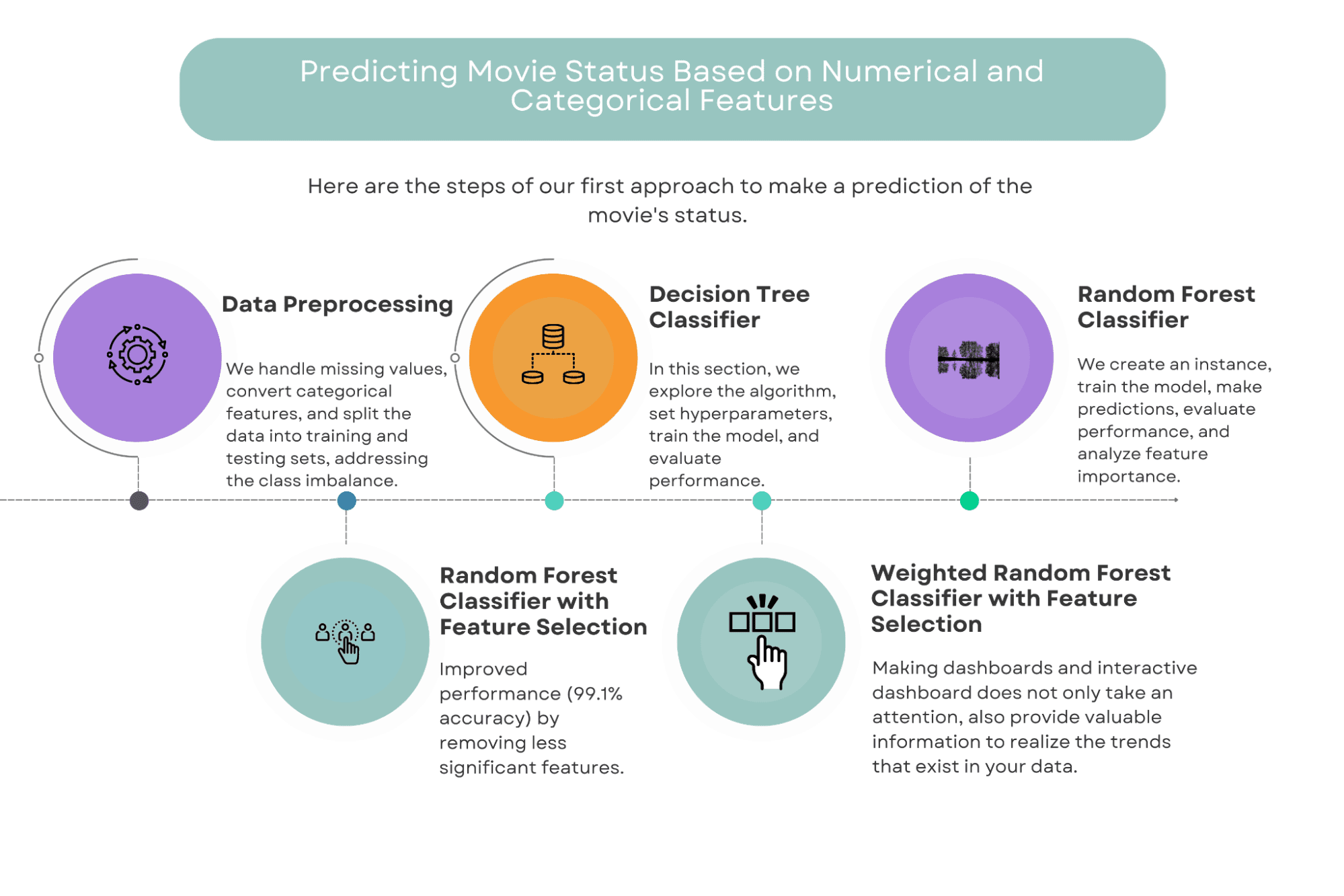
Data Science Project of Rotten Tomatoes Movie Rating Prediction: First Approach
Image by Author

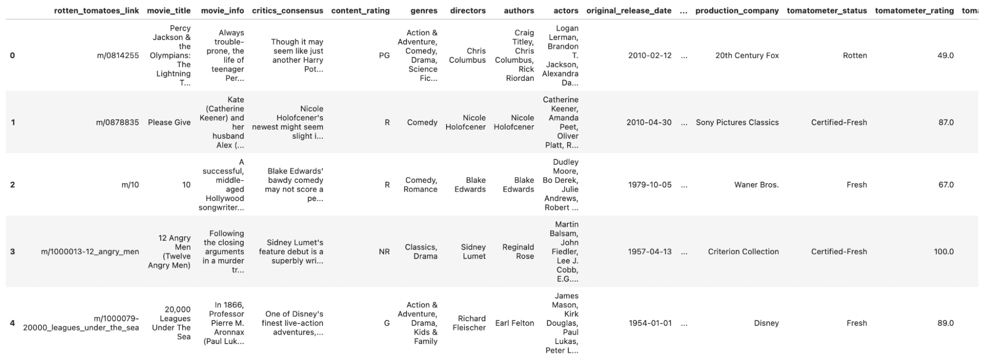
Let’s read our data and take a glimpse of it.

Here is the code.

df_movie = pd.read_csv('rotten_tomatoes_movies.csv')  df_movie.head()

Here is the output.

Data Science Project of Rotten Tomatoes Movie Rating Prediction: First Approach

Now, let’s start with Data Preprocessing.

There are many columns in our Data set.

Let’s see.

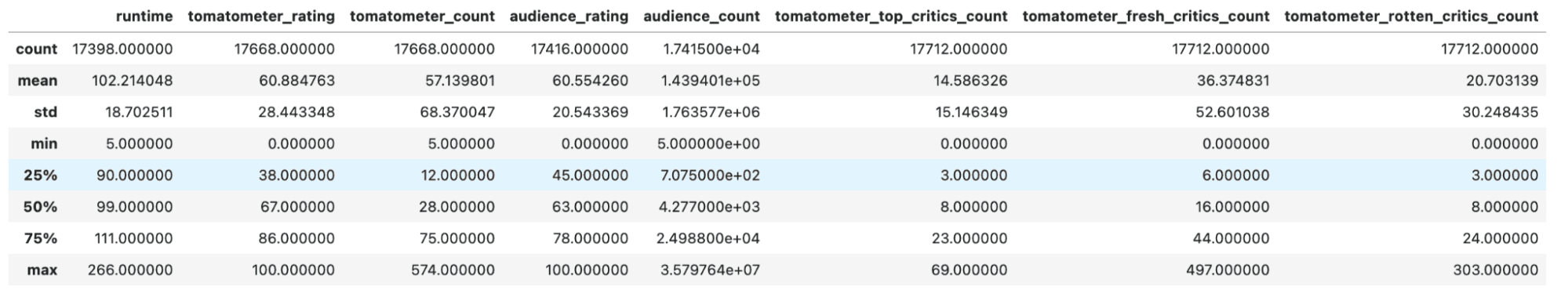
To develop a better understanding of the statistical features, let’s use describe the () method. Here is the code.

df_movie.describe()

Here is the output.

Data Science Project of Rotten Tomatoes Movie Rating Prediction: First Approach

Now, we have a quick overview of our data, let’s go to the preprocessing stage.

Data Preprocessing

Before we can begin building our models, it's essential to preprocess our data.

This involves cleaning the data by handling categorical features and converting them into numerical representations, and scaling the data to ensure that all features have equal importance.

We first examined the content_rating column to see the unique categories and their distribution in the dataset.

print(f'Content Rating category: {df_movie.content_rating.unique()}')

Then, we will create a bar plot to see the distribution of each content rating category.

ax = df_movie.content_rating.value_counts().plot(kind='bar', figsize=(12,9))  ax.bar_label(ax.containers[0])

Here is the full code.

print(f'Content Rating category: {df_movie.content_rating.unique()}')  ax = df_movie.content_rating.value_counts().plot(kind='bar', figsize=(12,9))  ax.bar_label(ax.containers[0])

Here is the output.

Data Science Project of Rotten Tomatoes Movie Rating Prediction: First Approach

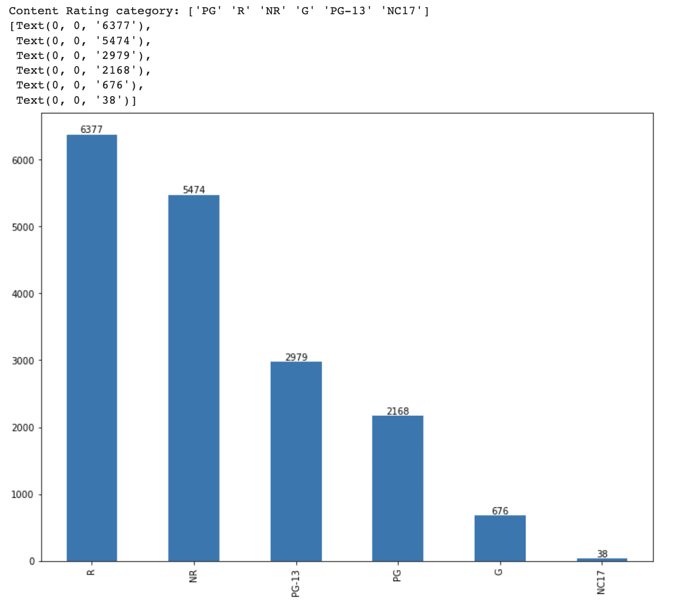
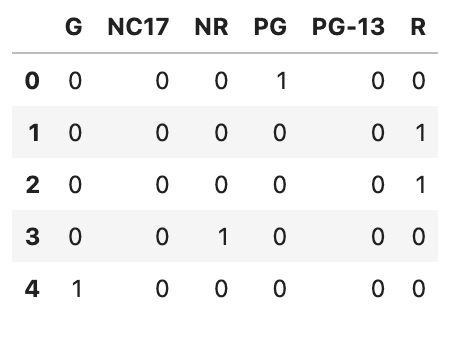
It is essential to convert categorical features into numeric forms for our machine learning models which need numeric inputs. For multiple elements in this data science project, we are going to apply two generally accepted methods: ordinal encoding and one-hot encoding. Ordinal encoding is better when categories imply a degree of intensity, but the one-hot encoding is ideal when no magnitude representation is provided. For the "content_rating" assets, we will use a one-hot encoding method.

Here is the code.

content_rating = pd.get_dummies(df_movie.content_rating)  content_rating.head()

Here is the output.

Data Science Project of Rotten Tomatoes Movie Rating Prediction: First Approach

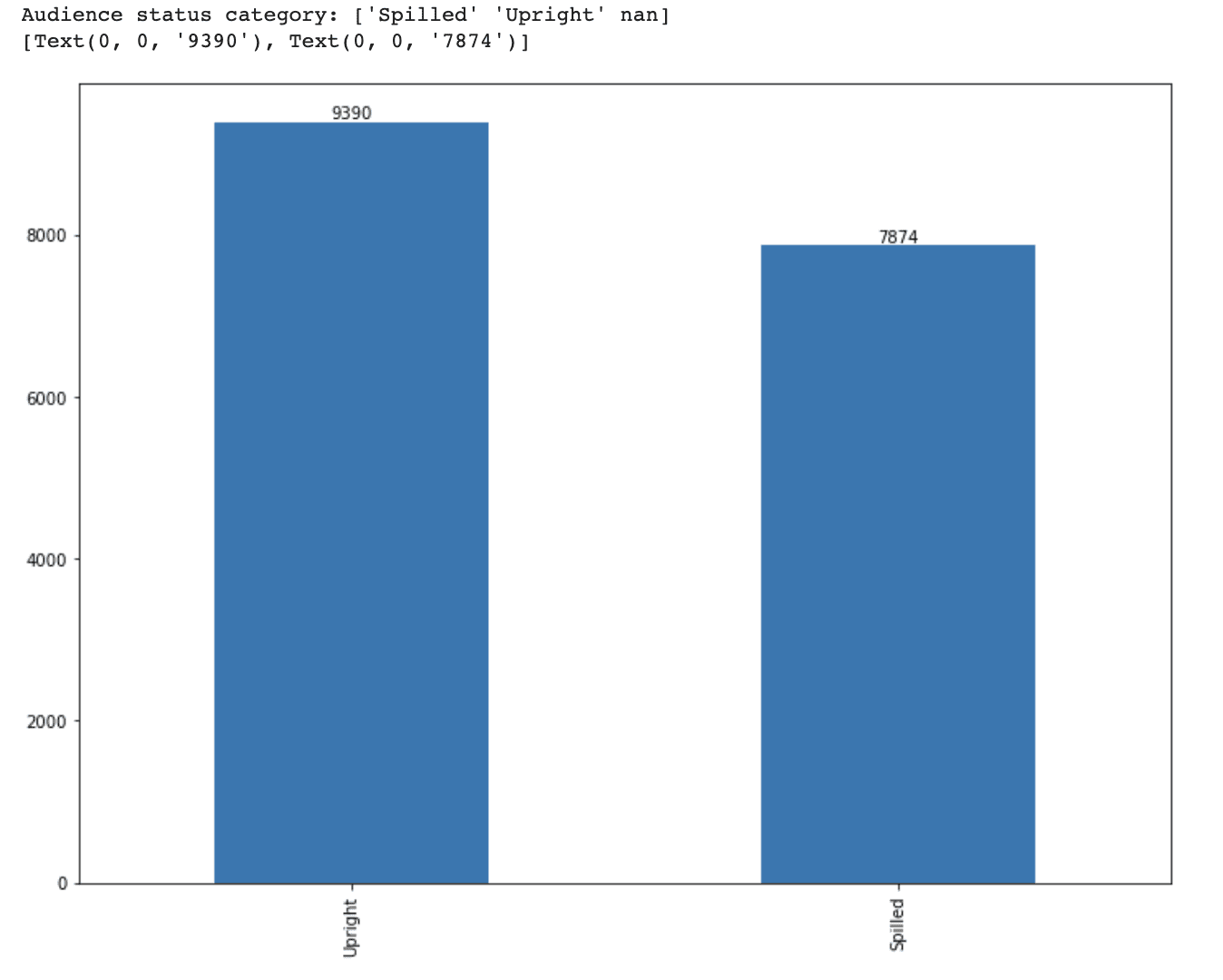
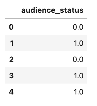
Let's go ahead and process another feature, audience_status.

This variable has two options: 'Spilled' and 'Upright'.

We did already apply one hot coding, so now it is time to transform this categorical variable into a numerical one by using ordinal encoding.

Because each category illustrates an order of magnitude, we will transform these into numerical values by using ordinal encoding.

As we did earlier, first let’s find the unique audience status.

print(f'Audience status category: {df_movie.audience_status.unique()}')

Then, let’s create a bar plot and print out the values on top of bars.

# Visualize the distribution of each category  ax = df_movie.audience_status.value_counts().plot(kind='bar', figsize=(12,9))  ax.bar_label(ax.containers[0])

Here is the full code.

print(f'Audience status category: {df_movie.audience_status.unique()}')  # Visualize the distribution of each category  ax = df_movie.audience_status.value_counts().plot(kind='bar', figsize=(12,9))  ax.bar_label(ax.containers[0])

Here is the output.

Data Science Project of Rotten Tomatoes Movie Rating Prediction: First Approach

Okay, now it is time to do ordinal coding by using replace method.

Then let’s view the first five rows by using the head() method.

Here is the code.

# Encode audience status variable with ordinal encoding  audience_status = pd.DataFrame(df_movie.audience_status.replace(['Spilled','Upright'],[0,1]))  audience_status.head()

Here is the output.

Data Science Project of Rotten Tomatoes Movie Rating Prediction: First Approach

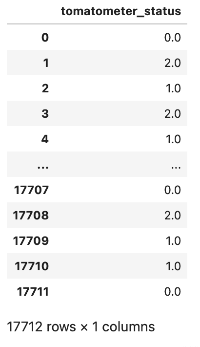
Since our target variable, tomatometer_status, have three distinct categories, 'Rotten', 'Fresh', and 'Certified-Fresh', these categories also represent an order of magnitude.

That’s why we again will do ordinal encoding to transform these categorical variables into numerical variables.

Here is the code.

# Encode tomatometer status variable with ordinal encoding  tomatometer_status = pd.DataFrame(df_movie.tomatometer_status.replace(['Rotten','Fresh','Certified-Fresh'],[0,1,2]))  tomatometer_status

Here is the output.

Data Science Project of Rotten Tomatoes Movie Rating Prediction: First Approach

After changing categorial to numerical, it is now time to combine the two data frames. We'll use Pandas pd.concat() function for this, and the dropna() method to remove rows with missing values across all columns.

Following that, we'll use the head function to look at the freshly formed DataFrame.

Here is the code.

df_feature = pd.concat([df_movie[['runtime', 'tomatometer_rating', 'tomatometer_count', 'audience_rating', 'audience_count', 'tomatometer_top_critics_count', 'tomatometer_fresh_critics_count', 'tomatometer_rotten_critics_count']], content_rating, audience_status, tomatometer_status], axis=1).dropna()  df_feature.head()

Here is the output.

Data Science Project of Rotten Tomatoes Movie Rating Prediction: First Approach

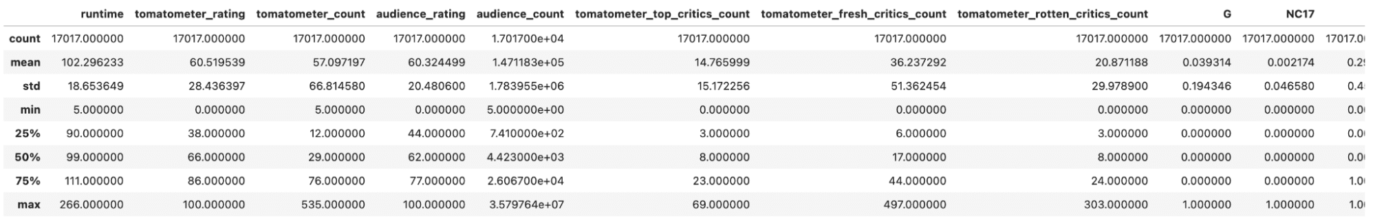
Great, now let’s inspect our numerical variables by using describe method.

Here is the code.

df_feature.describe()

Here is the output.

Data Science Project of Rotten Tomatoes Movie Rating Prediction: First Approach

Now let’s check the length of our DataFrame by using len method.

Here is the code.

len(df)

Here is the output.

Data Science Project of Rotten Tomatoes Movie Rating Prediction: First Approach

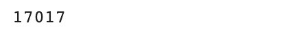
After removing rows with missing values and doing the transformation for building machine learning, now our data frame has 17017 rows.

Let’s now analyze the distribution of our target variables.

As we keep constantly doing since the beginning, we will draw a bar graph and put the values at the top of the bar.

Here is the code.

ax = df_feature.tomatometer_status.value_counts().plot(kind='bar', figsize=(12,9))  ax.bar_label(ax.containers[0])

Here is the output.

Data Science Project of Rotten Tomatoes Movie Rating Prediction: First Approach

Our dataset contains 7375 'Rotten,' 6475 'Fresh,' and 3167 'Certified-Fresh' films, indicating a class imbalance issue.

The problem will be addressed at a later time.

For the time being, let’s split our dataset into testing and training sets using an 80% to 20% split.

Here is the code.

X_train, X_test, y_train, y_test = train_test_split(df_feature.drop(['tomatometer_status'], axis=1), df_feature.tomatometer_status, test_size= 0.2, random_state=42)  print(f'Size of training data is {len(X_train)} and the size of test data is {len(X_test)}')

Here is the output.

Data Science Project of Rotten Tomatoes Movie Rating Prediction: First Approach

Decision Tree Classifier

In this section, we will look at the Decision Tree Classifier, a machine learning technique that is commonly used for classification problems and sometimes for regression.

The classifier works by dividing data points into branches, each of which has an inner node (which includes a set of conditions) and a leaf node (which has the predicted value).

Following these branches and considering the conditions (True or False), data points are separated into the proper categories. The process is seen below.
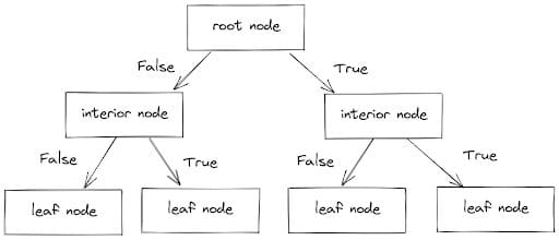
Data Science Project of Rotten Tomatoes Movie Rating Prediction: First Approach
Image by Author

When we apply a Decision Tree Classifier, we can alter multiple hyperparameters, like the maximum depth of the tree and the maximum number of leaf nodes.

For our first attempt, we will limit the number of leaf nodes to three in order to make the tree simple and understandable.

To begin, we will create a Decision Tree Classifier with a maximum of three leaf nodes. This classifier will then be trained on our training data and used to generate predictions on the test data. Finally, we will examine the accuracy, precision, and recall metrics to assess the performance of our limited Decision Tree Classifier.

Now let’s implement the Decision Tree algorithm with sci-kit learn step by step.

First, let’s define a Decision Tree Classifier object with a maximum of three leaf nodes, using the DecisionTreeClassifier() function from the scikit-learn library.

The random_state parameter is used to ensure that the same results are produced each time the code is run.

tree_3_leaf = DecisionTreeClassifier(max_leaf_nodes= 3, random_state=2)

Then it is time to train the Decision Tree Classifier on the training data (X_train and y_train), using the .fit() method.

tree_3_leaf.fit(X_train, y_train)

Next, we make predictions on the test data(X_test) using the trained classifier with the predict method.

y_predict = tree_3_leaf.predict(X_test)

Here we print the accuracy score and classification report of the predicted values compared to the actual target values of the test data. We use the accuracy_score() and classification_report() functions from the scikit-learn library.

print(accuracy_score(y_test, y_predict))  print(classification_report(y_test, y_predict))

Finally, we will plot the confusion matrix to visualize the performance of the Decision Tree Classifier on the test data. We use the plot_confusion_matrix() function from the scikit-learn library.

fig, ax = plt.subplots(figsize=(12, 9))  plot_confusion_matrix(tree_3_leaf, X_test, y_test, cmap='cividis', ax=ax)

Here is the code.

# Instantiate Decision Tree Classifier with max leaf nodes = 3  tree_3_leaf = DecisionTreeClassifier(max_leaf_nodes= 3, random_state=2)  # Train the classifier on the training data  tree_3_leaf.fit(X_train, y_train)  # Predict the test data with trained tree classifier  y_predict = tree_3_leaf.predict(X_test)  # Print accuracy and classification report on test data  print(accuracy_score(y_test, y_predict))  print(classification_report(y_test, y_predict))  # Plot confusion matrix on test data  fig, ax = plt.subplots(figsize=(12, 9))  plot_confusion_matrix(tree_3_leaf, X_test, y_test, cmap ='cividis', ax=ax)

Here is the output.

Data Science Project of Rotten Tomatoes Movie Rating Prediction: First Approach

It can be clearly seen from the output, our Decision Tree works well, especially taking into consideration that we limited it to three leaf nodes. One of the advantages of having a simple classifier is that the decision tree can be visualized and understandable.

Now, to understand how the decision tree makes decisions, let’s visualize the decision tree classifier by using the plot_tree method from sklearn.tree.

Here is the code.

fig, ax = plt.subplots(figsize=(12, 9))  plot_tree(tree_3_leaf, ax= ax)  plt.show()

Here is the output.

Data Science Project of Rotten Tomatoes Movie Rating Prediction: First Approach

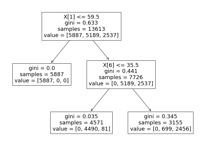
Now let’s analyze this decision tree, and find out how it carries out the decision-making process.

Specifically, the algorithm uses the 'tomatometer_rating' feature as the primary determinant of each test data point's classification.

  • If the 'tomatometer_rating' is less than or equal to 59.5, the data point is assigned a label of 0 ('Rotten'). Otherwise, the classifier progresses to the next branch.
  • In the second branch, the classifier uses the 'tomatometer_fresh_critics_count' feature to classify the remaining data points.
    • If the value of this feature is less than or equal to 35.5, the data point is labeled as 1 ('Fresh').
    • If not, it is labeled as 2 ('Certified-Fresh').

This decision-making process closely aligns with the rules and criteria that Rotten Tomatoes use to assign movie statuses.

According to the Rotten Tomatoes website, movies are classified as

  • ‘Fresh' if their tomatometer_rating is 60% or higher.
  • 'Rotten' if it falls below 60%.

Our Decision Tree Classifier follows a similar logic, classifying movies as 'Rotten' if their tomatometer_rating is below 59.5 and 'Fresh' otherwise.

However, when distinguishing between 'Fresh' and 'Certified-Fresh' movies, the classifier must consider several more features.

According to Rotten Tomatoes, films must meet specific criteria to be classified as 'Certified-Fresh', such as:

  • Having a consistent Tomatometer score of at least 75%
  • At least five reviews from top critics.
  • Minimum of 80 reviews for wide-release films.

Our limited Decision Tree model only takes into account the number of reviews from top critics to differentiate between 'Fresh' and 'Certified-Fresh' movies.

Now, we understand the logic behind the Decision Tree. So to increase its performance, let’s follow the same steps but this time, we will not add the max-leaf nodes argument.

Here is the step-by-step explanation of our code. This time I won't expand the code too much as we did before.

Define the decision tree classifier.

tree = DecisionTreeClassifier(random_state=2)

Train the classifier on the training data.

tree.fit(X_train, y_train)

Predict the test data with a trained tree classifier.

y_predict = tree.predict(X_test)

Print the accuracy and classification report.

print(accuracy_score(y_test, y_predict))  print(classification_report(y_test, y_predict))

Plot confusion matrix.

fig, ax = plt.subplots(figsize=(12, 9))  plot_confusion_matrix(tree, X_test, y_test, cmap ='cividis', ax=ax)

Great now, let’s see them together.

Here's the whole code.

fig, ax = plt.subplots(figsize=(12, 9))  # Instantiate Decision Tree Classifier with default hyperparameter settings  tree = DecisionTreeClassifier(random_state=2)    # Train the classifier on the training data  tree.fit(X_train, y_train)    # Predict the test data with trained tree classifier  y_predict = tree.predict(X_test)    # Print accuracy and classification report on test data  print(accuracy_score(y_test, y_predict))  print(classification_report(y_test, y_predict))    # Plot confusion matrix on test data  fig, ax = plt.subplots(figsize=(12, 9))  plot_confusion_matrix(tree, X_test, y_test, cmap ='cividis', ax=ax)

Here is the output.

Data Science Project of Rotten Tomatoes Movie Rating Prediction: First Approach

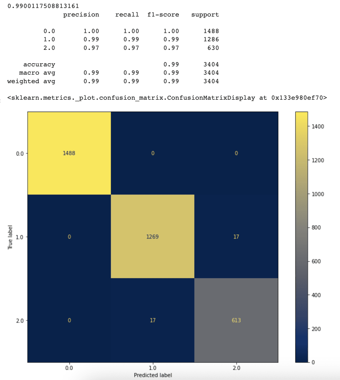
The accuracy, precision, and recall values of our classifier have increased as a result of removing the maximum leaf nodes limitation. The classifier now reaches 99% accuracy, up from 94% previously.

This displays that when we allow our classifier to pick the optimal number of leaf nodes on its own, it performs better.

Although the current result appears to be outstanding, more tuning to reach even better accuracy is still possible. In the next part, we'll look into this option.

Random Forest Classifier

Random Forest is an ensemble of Decision Tree Classifiers that have been combined into a single algorithm. It uses a bagging strategy to train each Decision Tree, which includes randomly picking training data points. Each tree is trained on a separate subset of the training data as a result of this technique.

The bagging method has become known for using a bootstrap methodology to sample data points, allowing the same data point to be picked for several Decision Trees.

Data Science Project of Rotten Tomatoes Movie Rating Prediction: First Approach
Image by Author

By using scikit learn, it is really easy to apply a Random forest classifier.

Using Scikit-learn to set up the Random Forest algorithm is an easy process.

The algorithm's performance, like the performance of the Decision Tree Classifier, may be increased through changing hyperparameter values such as the number of Decision Tree Classifiers, maximum leaf nodes, and maximum tree depth.

We will use default options here first.

Let’s see the code step-by-step again.

First, let’s instantiate a Random Forest Classifier object using the RandomForestClassifier() function from the scikit-learn library, with a random_state parameter set to 2 for reproducibility.

rf = RandomForestClassifier(random_state=2)

Then, train the Random Forest Classifier on the training data (X_train and y_train), using the .fit() method.

rf.fit(X_train, y_train)

Next, use the trained classifier to make predictions on the test data (X_test), using the .predict() method.

y_predict = rf.predict(X_test)

Then, print the accuracy score and classification report of the predicted values compared to the actual target values of the test data.

We use the accuracy_score() and classification_report() functions from the scikit-learn library again.

print(accuracy_score(y_test, y_predict))  print(classification_report(y_test, y_predict))  

Finally, let’s plot a confusion matrix to visualize the performance of the Random Forest Classifier on the test data. We use the plot_confusion_matrix() function from the scikit-learn library.

fig, ax = plt.subplots(figsize=(12, 9))  plot_confusion_matrix(rf, X_test, y_test, cmap ='cividis', ax=ax)

Here is the whole code.

# Instantiate Random Forest Classifier  rf = RandomForestClassifier(random_state=2)    # Train Random Forest Classifier on training data  rf.fit(X_train, y_train)    # Predict test data with trained model  y_predict = rf.predict(X_test)    # Print accuracy score and classification report  print(accuracy_score(y_test, y_predict))  print(classification_report(y_test, y_predict))    # Plot confusion matrix  fig, ax = plt.subplots(figsize=(12, 9))  plot_confusion_matrix(rf, X_test, y_test, cmap ='cividis', ax=ax)

Here is the output.

Data Science Project of Rotten Tomatoes Movie Rating Prediction: First Approach

The accuracy and confusion matrix results show that the Random Forest algorithm outperforms the Decision Tree Classifier. This shows the advantage of ensemble approaches such as Random Forest over individual classification algorithms.

Furthermore, tree-based machine learning methods allow us to identify the significance of each feature once the model has been trained. For this reason, Scikit-learn provides the feature_importances_ function.

Great, once again, let’s see the code step by step to understand it.

First, the feature_importances_ attribute of the Random Forest Classifier object is used to obtain the importance score of each feature in the dataset.

The importance score indicates how much each feature contributes to the prediction performance of the model.

# Get the feature importance  feature_importance = rf.feature_importances_

Next, the feature importances are printed out in descending order of importance, along with their corresponding feature names.

# Print feature importance  for i, feature in enumerate(X_train.columns):      print(f'{feature} = {feature_importance[i]}')

Then to visualize features from the most important to least important, let’s use argsort() method from the numpy.

# Visualize feature from the most important to the least important  indices = np.argsort(feature_importance)

Finally, a horizontal bar chart is created to visualize the feature importances, with features ranked from most to least important on the y-axis and the corresponding importance scores on the x-axis.

This chart allows us to easily identify the most important features in the dataset and to determine which features have the greatest impact on the model's performance.

plt.figure(figsize=(12,9))  plt.title('Feature Importances')  plt.barh(range(len(indices)), feature_importance[indices], color='b', align='center')  plt.yticks(range(len(indices)), [X_train.columns[i] for i in indices])  plt.xlabel('Relative Importance')  plt.show()

Here is the whole code.

# Get the fature importance  feature_importance = rf.feature_importances_    # Print feature importance  for i, feature in enumerate(X_train.columns):      print(f'{feature} = {feature_importance[i]}')    # Visualize feature from the most important to the least important  indices = np.argsort(feature_importance)    plt.figure(figsize=(12,9))  plt.title('Feature Importances')  plt.barh(range(len(indices)), feature_importance[indices], color='b', align='center')  plt.yticks(range(len(indices)), [X_train.columns[i] for i in indices])  plt.xlabel('Relative Importance')  plt.show()

Here is the output.

Data Science Project of Rotten Tomatoes Movie Rating Prediction: First Approach

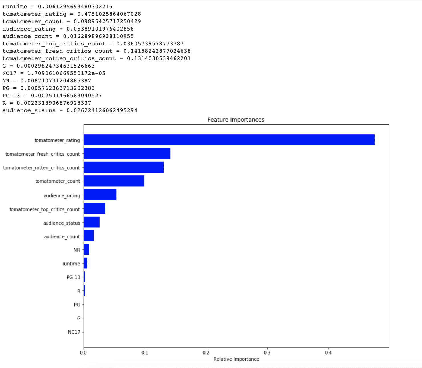
By seeing this graph, it is clear that NR, PG-13, R, and runtime did not consider important by the model for predicting unseen data points. In the next section, whether let’s see addressing this issue can increase our model's performance or not.

Random Forest Classifier with Feature Selection

Here is the code.

In the last section, we discovered that some of our features were considered less significant by our Random forest model, in making predictions.

As a result, to enhance the model’s performance, let’s exclude these less relevant features including NR, runtime, PG-13, R, PG, G, and NC17.

In the following code, we will get the feature importance first, then we will split to train and test set, but inside the code block we dropped these less significant features. Then we will print out the train and test set size.

Here is the code.

# Get the feature importance  feature_importance = rf.feature_importances_  X_train, X_test, y_train, y_test = train_test_split(df_feature.drop(['tomatometer_status', 'NR', 'runtime', 'PG-13', 'R', 'PG','G', 'NC17'], axis=1),df_feature.tomatometer_status, test_size= 0.2, random_state=42)  print(f'Size of training data is {len(X_train)} and the size of test data is {len(X_test)}')

Here is the output.

Data Science Project of Rotten Tomatoes Movie Rating Prediction: First Approach

Great, since we dropped these less significant features, let’s see whether our performance increased or not.

Because we did this too many times, I quickly explain the following codes.

In the following code, we first initialize a random forest classifier and then train the random forest on the training data.

rf = RandomForestClassifier(random_state=2)    rf.fit(X_train, y_train)

Then we calculate the accuracy score and classification report by using test data and print them out.

print(accuracy_score(y_test, y_predict))  print(classification_report(y_test, y_predict))

Finally, we plot the confusion matrix.

fig, ax = plt.subplots(figsize=(12, 9))  plot_confusion_matrix(rf, X_test, y_test, cmap ='cividis', ax=ax)

Here is the whole code.

# Initialize Random Forest class  rf = RandomForestClassifier(random_state=2)    # Train Random Forest on the training data after feature selection  rf.fit(X_train, y_train)    # Predict the trained model on the test data after feature selection  y_predict = rf.predict(X_test)    # Print the accuracy score and the classification report  print(accuracy_score(y_test, y_predict))  print(classification_report(y_test, y_predict))    # Plot the confusion matrix  fig, ax = plt.subplots(figsize=(12, 9))  plot_confusion_matrix(rf, X_test, y_test, cmap ='cividis', ax=ax)

Here is the output.

Data Science Project of Rotten Tomatoes Movie Rating Prediction: First Approach

It looks like our new approach works quite well.

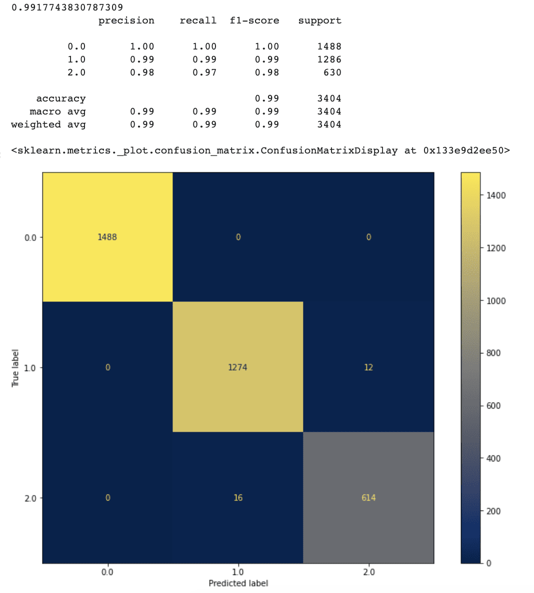
After doing feature selection, accuracy has increased to 99.1 %.

Our model's false positive and false negative rates have also lowered marginally when compared to the prior model.

This indicates that having more characteristics does not always imply a better model. Some insignificant characteristics may create noise which might be the reason for lowering the model's prediction accuracy.

Now since our model’s performance has increased that far, let’s discover other methods to check if we can increase more.

Weighted Random Forest Classifier with Feature Selection

In the first section, we realized that our features were a little imbalanced. We have three different values, Rotten' (represented by 0), 'Fresh' (represented by 1), and 'Certified-Fresh' (represented by 2).

First, let’s see the distribution of our features.

Here's the code for visualizing the label distribution.

ax = df_feature.tomatometer_status.value_counts().plot(kind='bar', figsize=(12,9))  ax.bar_label(ax.containers[0])

Here is the output.

Data Science Project of Rotten Tomatoes Movie Rating Prediction: First Approach

It is clear that the amount of data with the ‘Certified Fresh’ feature is much less than the others.

To solve the issue of data imbalance, we can use approaches such as the SMOTE algorithm to oversample the minority class or provide class weight information to the model during the training phase.

Here we will use the second approach.

To compute class weight, we will use the compute_class_weight() function from the scikit-learn library.

Inside this function, the class_weight parameter is set to 'balanced' to account for imbalanced classes, and the classes parameter is set to the unique values in the tomatometer_status column of df_feature.

The y parameter is set to the values of the tomatometer_status column in df_feature.

class_weight = compute_class_weight(class_weight= 'balanced', classes= np.unique(df_feature.tomatometer_status),                         y = df_feature.tomatometer_status.values)

Then, the dictionary is created to map the class weights to their respective indices.

This is done by converting the class weight list to a dictionary using the dict() function and zip() function.

The range() function is used to generate a sequence of integers corresponding to the length of the class weight list, which is then used as the keys for the dictionary.

class_weight_dict = dict(zip(range(len(class_weight.tolist())), class_weight.tolist()

Finally, let’s see our dictionary.

class_weight_dict

Here is the whole code.

class_weight = compute_class_weight(class_weight= 'balanced', classes= np.unique(df_feature.tomatometer_status),                         y = df_feature.tomatometer_status.values)    class_weight_dict = dict(zip(range(len(class_weight.tolist())), class_weight.tolist()))  class_weight_dict

Here is the output.

Data Science Project of Rotten Tomatoes Movie Rating Prediction: First Approach

Class 0 ('Rotten') has the least weight, while class 2 ('Certified-Fresh') has the highest weight.

When we apply our Random Forest classifier, we can now include this weight information as an argument.

The remaining code is the same as we did earlier many times.

Let's build a new Random Forest model with class weight data, train it on the training set, predict the test data, and display the accuracy score and confusion matrix.

Here is the code.

# Initialize Random Forest model with weight information  rf_weighted = RandomForestClassifier(random_state=2, class_weight=class_weight_dict)    # Train the model on the training data  rf_weighted.fit(X_train, y_train)    # Predict the test data with the trained model  y_predict = rf_weighted.predict(X_test)    #Print accuracy score and classification report  print(accuracy_score(y_test, y_predict))  print(classification_report(y_test, y_predict))    #Plot confusion matrix  fig, ax = plt.subplots(figsize=(12, 9))  plot_confusion_matrix(rf_weighted, X_test, y_test, cmap ='cividis', ax=ax)

Here is the output.

Data Science Project of Rotten Tomatoes Movie Rating Prediction: First Approach

Our model's performance increased when we added class weights, and it now has an accuracy of 99.2%.

The number of correct predictions for the “Fresh “ label also increased by one.

Using class weights to address the data imbalance problem is a useful method since it encourages our model to pay more attention to labels with higher weights throughout the training phase.

Link to this data science project: https://platform.stratascratch.com/data-projects/rotten-tomatoes-movies-rating-prediction

Nate Rosidi is a data scientist and in product strategy. He's also an adjunct professor teaching analytics, and is the founder of StrataScratch, a platform helping data scientists prepare for their interviews with real interview questions from top companies. Connect with him on Twitter: StrataScratch or LinkedIn.

More On This Topic

  • KDnuggets™ News 20:n44, Nov 18: How to Acquire the Most Wanted Data…
  • How to Future-Proof Your Data Science Project
  • Data Science Project Infrastructure: How To Create It
  • 19 Data Science Project Ideas for Beginners
  • 4 Steps for Managing a Data Science Project
  • 7 Tips for Data Science Project Management

Want To Understand Machine Learning? Here’s A Beginner-Friendly Way To Start

Stream of binary codes.
Image: StackCommerce

What was once sci-fi is quickly becoming an ordinary — and vital — part of everyday life. Artificial intelligence has changed the way we do business, make decisions, and even interact with one another. While the average person isn’t expected to be an expert on machine learning or AI by any means, it never hurts to be informed about the technologies shaping the future. And that’s why The 2023 Machine Learning for Absolute Beginners E-Degree Program is so valuable.

This extensive program gives you 35 hours of certification training designed for machine learning novices. The program is taught by Eduonix Learning Solutions, a premier training and skill development organization designed by experts in their fields.

This beginner-friendly e-degree covers some of the most basic tools and technologies of machine learning, like Python, NumPy, SciPy, Pandas, and Matplotlib. You’ll understand the many libraries of Python, learn the basics of Python programming, and understand how this general-purpose language has become foundational for AI and ML. You’ll learn techniques for data collection, processing, and visualization, how to master inferential statistics and hypothesis testing, develop regression analysis and prediction skills, and much more. Throughout the course, you’ll touch on a variety of machine learning algorithms for many applications as you work through real-life projects to predict the housing market, predict stock prices, and more. You might even put yourself on track for a career in machine learning.

By the end of the bundle, you’ll have completed five projects and get a series of quizzes to fortify your learning. When all’s said and done, you’ll earn a certificate of completion to demonstrate your expertise.

Take your skills into 2023 and beyond. For a limited time, you can get The 2023 Machine Learning for Absolute Beginners E-Degree Program at 90% off $300 for just $29.99.

Prices and availability are subject to change.

Subscribe to the Innovation Insider Newsletter

Catch up on the latest tech innovations that are changing the world, including IoT, 5G, the latest about phones, security, smart cities, AI, robotics, and more.

Delivered Tuesdays and Fridays Sign up today

10 Best Vector Database for Building LLMs

10 Best Vector Database for Building LLMs

First and foremost, vector databases enable faster processing of large datasets. These databases are specifically designed to store and retrieve data efficiently, resulting in accelerated processing times. By leveraging the power of vector representations, LLMs can quickly analyse and comprehend vast amounts of information, leading to improved efficiency and reduced processing times.

Scalability is another crucial aspect facilitated by vector databases. These databases can seamlessly scale up or down based on the user’s requirements, making them capable of efficiently managing massive volumes of data without compromising performance. This scalability empowers LLMs to handle diverse and evolving datasets, ensuring their effectiveness in dynamic environments and accommodating the growing demands of users.

The precise similarity matching capability offered by vector databases is essential for various applications, particularly in voice and image recognition. By representing audio and visual data as vectors, LLMs can accurately identify and match similar items, enabling highly accurate voice and image recognition functionalities.

Additionally, vector databases enhance search capabilities through the utilisation of advanced search algorithms. With these databases, LLMs can provide more effective and relevant search results, enabling users to access the desired information efficiently. This improvement in search efficiency contributes to a more seamless and user-friendly experience for individuals interacting with LLM-based applications.

Now that we know the importance and capabilities of vector database, here is a list of best vector database options for LLMs –

MongoDB

Firstly, MongoDB, the developer’s favourite database, has come up with Atlas Vector Search. This NoSQL database has recently incorporated vector search capabilities, revolutionising the integration of generative AI and semantic search into applications. By combining the power of MongoDB with vector search, developers can unlock new possibilities in data analysis, recommendation systems, and natural language processing.

With Atlas Vector Search, developers have the ability to conduct searches on unstructured data effortlessly. It enables them to generate vector embeddings using your preferred machine learning model, whether it’s OpenAI, Hugging Face, or others, and store them directly in Atlas. This powerful feature supports a wide range of use cases, including similarity search, recommendation engines, Q&A systems, dynamic personalization, and long-term memory for LLMs.

DataStax

DataStax had recently introduced AstraDB, a vector database designed to streamline app development processes, allowing developers to create applications faster and more efficiently. By integrating with AstraDB, which handles Cassandra operations, AppCloudDB frees developers from the complexities of database management, enabling them to focus on app creation. It simplifies every step of the development process by eliminating time-consuming configuration changes, allowing developers to dedicate their time to writing code that matters.

Developers can improve app performance across any cloud environment without the need to scale up or down manually. It provides a seamless and scalable solution, ensuring that applications perform optimally without the hassle of performance optimization and cloud infrastructure management. AstraDB enables developers to accelerate the app development cycle, simplify workflows, and deliver high-performing applications efficiently.

Milvus

Milvus is a vector database system designed for efficient handling of complex data. It offers high speed and performance for data retrieval and analysis, making it ideal for applications that require quick insights. Milvus can handle massive datasets effectively, simplifying the storage and analysis of large volumes of data.

It supports multiple vector data formats, including audio, text, and images, allowing flexibility in data representation. The comprehensive indexing capabilities of Milvus enable fast and accurate vector similarity searches, enhancing the precision of search results. It also enables real-time updates, ensuring the availability of the most recent data for analysis.

Weaviate

Weaviate is a powerful and user-friendly database that specialises in storing and searching high-dimensional vectors. It introduces semantic search, enabling users to find related objects based on meaning and context rather than just keywords. Weaviate supports real-time updates, keeping the database up-to-date with the latest changes. Its flexible schema allows easy adaptation to different data types and structures.

Being an open-source solution, Weaviate offers visibility and customization options to meet specific needs. It provides personalised suggestions by analysing user queries, improving the user experience. Integration with deep learning frameworks makes it suitable for image or text categorization tasks, and its time series analysis capabilities make it effective for forecasting and anomaly detection projects.

Pinecone

Pinecone is a robust vector database known for its impressive speed, scalability, and support for complex data. It excels at fast and efficient data retrieval, making it ideal for applications that require quick access to vectors. Pinecone can handle large data volumes, making it suitable for big projects and enabling the detection of patterns and irregularities in large datasets. Real-time updates ensure that the database is continuously up-to-date.

It is optimised for high-dimensional data types such as text, enhancing the understanding and search capabilities for complex data. Pinecone’s automatic indexing feature speeds up searches, enabling efficient similarity search for grouping and recommendations. Additionally, Pinecone provides capabilities for identifying unusual behaviour in time-series data, making it valuable for anomaly detection.

RedisVector

RedisVector is a vector database that focuses on efficient processing of vector data. It excels at storing and analysing large amounts of vector data, including tensors, matrices, and numerical arrays. By leveraging Redis, an in-memory data store, RedisVector delivers high-performance query response times. It offers built-in indexing and search capabilities, enabling quick searching and finding similar vectors.

RedisVector supports various distance measures for comparing vectors and performing complex analytical operations. With its operations on vector data, including element-wise arithmetic and aggregation, RedisVector provides a versatile environment for working with vectors. It is particularly suited for machine learning applications that process and analyse high-dimensional vector data, enabling the creation of customised recommendation systems and accurate similarity-based search.

SingleStore

SingleStore is a scalable database that excels in data processing and high-performance analytics. It can handle large amounts of data by scaling horizontally across multiple nodes, ensuring high availability and scalability. SingleStore leverages in-memory technology for quick data processing and analysis. It enables real-time analytics, allowing users to interpret and analyse data in real-time, facilitating quick decision-making.

The full SQL support of SingleStore enables easy interaction with the database using common SQL queries. It supports continuous data pipelines, facilitating smooth data intake from various sources. SingleStore also integrates with machine learning tools and libraries, enabling advanced analytics. Its efficient management of time series data makes it suitable for applications such as IoT, banking, and monitoring.

Relevance AI

Relevance AI is a comprehensive vector database designed for storing, searching, and analysing large amounts of data. It offers fast query response times, allowing users to retrieve insights from data quickly. With advanced algorithms, Relevance AI delivers precise and relevant search results. It supports various data types and formats, making it versatile for working with different datasets.

Real-time search capabilities enable instant access to the desired information. Relevance AI is capable of handling both small and large amounts of data, making it suitable for a wide range of applications. By leveraging user preferences and historical data, it can create personalised experiences for users, enhancing engagement and satisfaction.

Qdrant

Qdrant is a versatile vector database solution that excels in effective data management and analysis. It offers advanced search techniques for finding similar objects in a dataset, enabling efficient retrieval of related items. Qdrant’s scalability allows it to handle increasing amounts of data without compromising performance. It supports real-time updates and indexing, ensuring that the database remains up-to-date and searchable.

With various query options, including filters, aggregations, and sorting, Qdrant provides flexibility in data exploration. It is particularly useful for similarity-based suggestions, anomaly detection, and image/text search applications.

Vespa.ai

Vespa.ai is a vector database known for its quick query results and real-time analytics capabilities. By integrating ML algorithms, Vespa.ai enables advanced data analysis and predictive modelling. The high data availability and fault tolerance of Vespa.ai ensure continuous service and minimal downtime.

Customisable ranking options allow organisations to prioritise and obtain the most relevant data. Vespa.ai supports geospatial search, enabling location-based searches for spatial applications. It is particularly suitable for media and content-driven applications, providing targeted ads and real-time statistics for improved audience targeting.

The post 10 Best Vector Database for Building LLMs appeared first on Analytics India Magazine.

ChatGPT on iPhone Can Now “Browse with Bing”

iPhone Users Can Now Use ChatGPT with Internet

Last month, OpenAI announced the release of its ChatGPT for iOS users. Now, to take the capabilities of its chatbot even further, the company has announced that the chatbot will also be able to access the internet through Bing Search.

The new feature is only available for ChatGPT Plus users at the moment, which comes with a $20 subscription per month. “Plus users can now use Browsing to get comprehensive answers and current insights on events and information that extend beyond the model’s original training data,” reads the release notes.

To try it out, users have to enable Browsing in the “new features” settings section. Then select GPT-4 in the model switcher and choose “Browse with Bing” in the drop-down menu.

Now users can finally move over the chatbots limitation of the knowledge cutoff of 2021. This was earlier achieved by introducing plugins for ChatGPT on the browser interface.

The company has also released improvements in search history. Now, users can browse their past conversations better and more seamlessly. Android users still wait for a ChatGPT app while OpenAI’s blog says, “P.S. Android users, you’re next!.”

This comes after OpenAI said that users can now create and share ChatGPT conversations using shared links. Recipients can view or copy the conversation to continue the discussion. This feature is still in Alpha tests within a small group and will be rolled out to all users in the next few weeks.

This all comes in the backdrop of OpenAI planning to release its own marketplace for AI models built on top of its technology. Possibly, by making ChatGPT on iOS the capabilities of browning the internet, OpenAI wants its own app to stand out in its own marketplace of AI apps.

The post ChatGPT on iPhone Can Now “Browse with Bing” appeared first on Analytics India Magazine.

Bengaluru Researcher’s Model Accurately Spots AI-generated Profile Pictures 

IIT-Kharagpur alumni, Shivansh Mundra, who currently works at Linkedin, alongside researchers from University of California and Berkeley, recently came up with a new technique to accurately identify the fake profile images generated by GAN (generative adversarial network).

Mundra told AIM “When we studied thousands of profile pictures we found specific structural patterns in the ones generated by Gan. This information was really useful to us, and what we did is we created a very simple model, simple as a linear model.” he said.

The research collaboration by UC Berkeley and Linkedin used light-weight, low-dimensional models with relatively minimal training data that mathematically computes the definite pattern of StyleGAN faces from real profile images.

The Rise of Fake Profile Images

Linkedin which hosts more than 930 million profiles, professionally connecting each other is also home to hundreds of thousands of fake profiles masquerading as real ones. They prey on unsuspecting users, offering jobs that don’t exist, fake tech support in exchange for money or just traditional phishing.

The first step in social media scams is falling for the profile picture. There are tools that help in finding if the picture is GAN generated or real but they’re only about 60% accurate. The research collaboration by UC Berkeley and Linkedin accurately identifies artificially generated profile pictures 99.6% of the time while misidentifying genuine pictures as fake only 1%.

How does it work?

Most models done so far solves the problem of identifying fake images using convolutional neural networks or CNN, a type of deep learning model which involves a filter. The image is passed through this filter to pick out the distinct structure or pattern. By using multiple filters you can pick out various specific features. This is effective only when there is a large training data for the model to learn the common features of a GAN image.

The downside to this is that GAN with its adversarial features, outperforms itself. “The generated images have patterns which repeat themselves, and there is less diversity in the 100,000 images we studied. The synthetic images are very structural and this information was really useful to us. With this in mind, we created a very simple model, as simple as a linear model,” explained Mundra.

Other methods

When it comes to addressing this issue, there are generally two forensic methods that can be used. The first is a hypothesis-based approach, which detects irregularities in synthetically created faces. However, this method faces challenges when dealing with advanced synthesis engines that can mimic genuine features. The other, data-driven methods, such as machine learning, can distinguish between natural faces and computer-generated ones. Nonetheless, they may struggle when confronted with unfamiliar images.

The proposed approach in this paper takes a hybrid approach, combining both methods. It starts by identifying a distinctive geometric attribute in computer-generated faces and then employs data-driven techniques for measurement and detection. This approach relies on a lightweight and easily trainable classifier, requiring training on a small set of synthetic faces.

Mundra said that to accomplish this, they created 41,500 synthetic faces using five different synthesis engines, in addition to an extra dataset containing 100,000 real LinkedIn profile pictures.

The previous accuracy rate extends only to human faces produced by GAN generators though they’re working on models that would pick up fake images generated by stable diffusion and other tools.

What’s next?

“This is just for the GAN based images, in other methods like diffusion or these new transformer based methods like Stable Diffusion, which have different types of structural patterns built in them, we weren’t able to detect fake images with these simple linear models. But there are other methods which we are working on which we’ll probably put them out soon,” Shivansh explained.

The post Bengaluru Researcher’s Model Accurately Spots AI-generated Profile Pictures appeared first on Analytics India Magazine.