Рубрика: AI

The problem of image-based sexual abuse through non-consensual deepfake pornography has always been a problem. But now with hyper-realistic generative image models like Stable Difussion, Midjourney, and alike, it is easier than ever.

But we don’t have any strict laws to protect the victim from the mishap. However, to get a quick and easy solution, in a scenario where an individual employs AI or Photoshop to manipulate your image into a nude photo, you can take steps to address this situation by visiting StopNCII. This is available worldwide.

You can upload both the original and altered versions of the photo. Once submitted, the altered image will be effectively removed from all online platforms, and you won’t need to engage in direct communication. Your privacy will be fully safeguarded.

How Are They Doing This?

Back in 2021, Meta, along with 50 other global NGOs, aided UK Revenge Porn Helpline in launching StopNCII.org. It combats online non-consensual sharing of private images, empowering global users to proactively secure intimate images on tech platforms using on-device hashing for safety and privacy.

The tool employs advanced hash-generating technology, assigning a unique numerical code to images to create a secure digital fingerprint. Tech companies involved with StopNCII.org use these hashes to detect sharing of these images on their platforms.

Participating companies use the hashes from StopNCII.org to identify shared images on their platforms, ensuring the original images remain on the user’s device. Only hashes, not the images, are shared with StopNCII.org and tech platforms, preventing further distribution of sensitive content and maintaining ownership.

StopNCII.org aids adults over 18 concerned about the non-consensual sharing of intimate images. For those under 18, alternative resources like the National Center for Missing & Exploited Children (NCMEC) provide appropriate support.

Vicious Loop of Deepfakes

Accordning to a report, 96% of nonconsensual deepfake videos online involve women, primarily celebrities, transformed into sexual content without their permission.

“The rise of AI-generated porn and deepfake porn normalises the use of a woman’s image or likeness without her consent,” Sophie Maddocks, a researcher at the University of Pennsylvania tracking image-based sexual abuse, told AFP.

Emma Watson, Kristen Bell, Natalie Portman, Taylor Swift and other actors have been through this. However, it is not restricted to celebrities.

Indian Journalist Rana Ayyub revealed in a terrifying post how she became the victim of deep fake porn after she took a stand on the Kathua gang rape in 2018. American Twitch streamer who goes by the gaming name QTCinderella became the latest victim of deepfake porn as she was harassed by people sending her copies of the deep fakes depicting her.

Read more about StopNCII here. Stay safe.

The post Combat AI-Generated Nude Photos with StopNCII appeared first on Analytics India Magazine.

MetaGPT, a Multi-Agent Framework on Github, approaching 10,000 stars, is looking to transform the landscape of software development. This groundbreaking framework takes a single-line requirement as input and delivers a spectrum of outputs, including user stories, competitive analysis, requirements, data structures, APIs, and documents.

Behind the scenes, MetaGPT harnesses the power of product managers, architects, project managers, and engineers, all collaboratively working within its virtual environment. This cohesive orchestration mirrors the entire software development process, incorporating meticulously crafted Standard Operating Procedures (SOPs).

Drawing inspiration from the core philosophy of Code = SOP(Team), MetaGPT propels software development to new heights. By assigning roles to its AI agents, such as product managers, architects, project managers, and engineers, MetaGPT emulates the dynamics of a full-fledged software company.

Astonishingly, a mere $0.2, covering the GPT-4 API costs, enables the generation of a comprehensive example complete with analysis and design. For more extensive projects, the investment amounts to around $2.0.

MetaGPT’s prowess lies in its ability to create a collaborative software entity, seamlessly executing intricate tasks. With MetaGPT, the future of software development has arrived, ushering in a new era of efficiency and innovation.
Github Repository: https://github.com/geekan/MetaGPT

The post MetaGPT Lets You Create Your Own Virtual Software Company appeared first on Analytics India Magazine.

Image by Editor

As Karl Pearson, a British mathematician has once stated, Statistics is the grammar of science and this holds especially for Computer and Information Sciences, Physical Science, and Biological Science. When you are getting started with your journey in Data Science or Data Analytics, having statistical knowledge will help you to better leverage data insights.

“Statistics is the grammar of science.” Karl Pearson

The importance of statistics in data science and data analytics cannot be underestimated. Statistics provides tools and methods to find structure and to give deeper data insights. Both Statistics and Mathematics love facts and hate guesses. Knowing the fundamentals of these two important subjects will allow you to think critically, and be creative when using the data to solve business problems and make data-driven decisions. In this article, I will cover the following Statistics topics for data science and data analytics:

- Random variables    - Probability distribution functions (PDFs)    - Mean, Variance, Standard Deviation    - Covariance and Correlation     - Bayes Theorem    - Linear Regression and Ordinary Least Squares (OLS)    - Gauss-Markov Theorem    - Parameter properties (Bias, Consistency, Efficiency)    - Confidence intervals    - Hypothesis testing    - Statistical significance     - Type I & Type II Errors    - Statistical tests (Student's t-test, F-test)    - p-value and its limitations    - Inferential Statistics     - Central Limit Theorem & Law of Large Numbers    - Dimensionality reduction techniques (PCA, FA)

If you have no prior Statistical knowledge and you want to identify and learn the essential statistical concepts from the scratch, to prepare for your job interviews, then this article is for you. This article will also be a good read for anyone who wants to refresh his/her statistical knowledge.

Before we start, welcome to LunarTech!

Welcome to LunarTech.ai, where we understand the power of job-searching strategies in the dynamic field of Data Science and AI. We dive deep into the tactics and strategies required to navigate the competitive job search process. Whether it’s defining your career goals, customizing application materials, or leveraging job boards and networking, our insights provide the guidance you need to land your dream job.

Preparing for data science interviews? Fear not! We shine a light on the intricacies of the interview process, equipping you with the knowledge and preparation necessary to increase your chances of success. From initial phone screenings to technical assessments, technical interviews, and behavioral interviews, we leave no stone unturned.

At LunarTech.ai, we go beyond the theory. We’re your springboard to unparalleled success in the tech and data science realm. Our comprehensive learning journey is tailored to fit seamlessly into your lifestyle, allowing you to strike the perfect balance between personal and professional commitments while acquiring cutting-edge skills. With our dedication to your career growth, including job placement assistance, expert resume building, and interview preparation, you’ll emerge as an industry-ready powerhouse.

Join our community of ambitious individuals today and embark on this thrilling data science journey together. With LunarTech.ai, the future is bright, and you hold the keys to unlock boundless opportunities.

Random Variables

The concept of random variables forms the cornerstone of many statistical concepts. It might be hard to digest its formal mathematical definition but simply put, a random variable is a way to map the outcomes of random processes, such as flipping a coin or rolling a dice, to numbers. For instance, we can define the random process of flipping a coin by random variable X which takes a value 1 if the outcome if heads and 0 if the outcome is tails.

In this example, we have a random process of flipping a coin where this experiment can produce two possible outcomes: {0,1}. This set of all possible outcomes is called the sample space of the experiment. Each time the random process is repeated, it is referred to as an event. In this example, flipping a coin and getting a tail as an outcome is an event. The chance or the likelihood of this event occurring with a particular outcome is called the probability of that event. A probability of an event is the likelihood that a random variable takes a specific value of x which can be described by P(x). In the example of flipping a coin, the likelihood of getting heads or tails is the same, that is 0.5 or 50%. So we have the following setting:

where the probability of an event, in this example, can only take values in the range [0,1].

The importance of statistics in data science and data analytics cannot be underestimated. Statistics provides tools and methods to find structure and to give deeper data insights.

Mean, Variance, Standard Deviation

To understand the concepts of mean, variance, and many other statistical topics, it is important to learn the concepts of population and sample. The population is the set of all observations (individuals, objects, events, or procedures) and is usually very large and diverse, whereas a sampleis a subset of observations from the population that ideally is a true representation of the population.

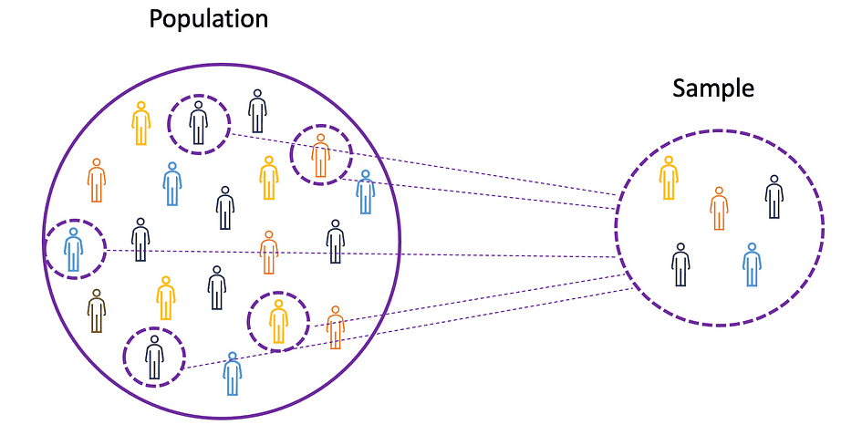
Image Source: The Author

Given that experimenting with an entire population is either impossible or simply too expensive, researchers or analysts use samples rather than the entire population in their experiments or trials. To make sure that the experimental results are reliable and hold for the entire population, the sample needs to be a true representation of the population. That is, the sample needs to be unbiased. For this purpose, one can use statistical sampling techniques such as Random Sampling, Systematic Sampling, Clustered Sampling, Weighted Sampling, and Stratified Sampling.

Mean

The mean, also known as the average, is a central value of a finite set of numbers. Let’s assume a random variable X in the data has the following values:

where N is the number of observations or data points in the sample set or simply the data frequency. Then the sample meandefined by ?, which is very often used to approximate the population mean, can be expressed as follows:

The mean is also referred to as expectation which is often defined by E() or random variable with a bar on the top. For example, the expectation of random variables X and Y, that is E(X) and E(Y), respectively, can be expressed as follows:

import numpy as np  import math  x = np.array([1,3,5,6])  mean_x = np.mean(x)  # in case the data contains Nan values  x_nan = np.array([1,3,5,6, math.nan])  mean_x_nan = np.nanmean(x_nan)

Variance

The variance measures how far the data points are spread out from the average value, and is equal to the sum of squares of differences between the data values and the average (the mean). Furthermore, the population variance, can be expressed as follows:

x = np.array([1,3,5,6])  variance_x = np.var(x)    # here you need to specify the degrees of freedom (df) max number of logically independent data points that have freedom to vary  x_nan = np.array([1,3,5,6, math.nan])  mean_x_nan = np.nanvar(x_nan, ddof = 1)

For deriving expectations and variances of different popular probability distribution functions, check out this Github repo.

Standard Deviation

The standard deviation is simply the square root of the variance and measures the extent to which data varies from its mean. The standard deviation defined by sigmacan be expressed as follows:

Standard deviation is often preferred over the variance because it has the same unit as the data points, which means you can interpret it more easily.

x = np.array([1,3,5,6])  variance_x = np.std(x)    x_nan = np.array([1,3,5,6, math.nan])  mean_x_nan = np.nanstd(x_nan, ddof = 1)

Covariance

The covariance is a measure of the joint variability of two random variables and describes the relationship between these two variables. It is defined as the expected value of the product of the two random variables’ deviations from their means. The covariance between two random variables X and Z can be described by the following expression, where E(X) and E(Z) represent the means of X and Z, respectively.

Covariance can take negative or positive values as well as value 0. A positive value of covariance indicates that two random variables tend to vary in the same direction, whereas a negative value suggests that these variables vary in opposite directions. Finally, the value 0 means that they don’t vary together.

x = np.array([1,3,5,6])  y = np.array([-2,-4,-5,-6])  #this will return the covariance matrix of x,y containing x_variance, y_variance on diagonal elements and covariance of x,y  cov_xy = np.cov(x,y)

Correlation

The correlation is also a measure for relationship and it measures both the strength and the direction of the linear relationship between two variables. If a correlation is detected then it means that there is a relationship or a pattern between the values of two target variables. Correlation between two random variables X and Z are equal to the covariance between these two variables divided to the product of the standard deviations of these variables which can be described by the following expression.

Correlation coefficients’ values range between -1 and 1. Keep in mind that the correlation of a variable with itself is always 1, that is Cor(X, X) = 1. Another thing to keep in mind when interpreting correlation is to not confuse it with causation, given that a correlation is not causation. Even if there is a correlation between two variables, you cannot conclude that one variable causes a change in the other. This relationship could be coincidental, or a third factor might be causing both variables to change.

x = np.array([1,3,5,6])  y = np.array([-2,-4,-5,-6])  corr = np.corrcoef(x,y)

Probability Distribution Functions

A function that describes all the possible values, the sample space, and the corresponding probabilities that a random variable can take within a given range, bounded between the minimum and maximum possible values, is called a probability distribution function (pdf) or probability density. Every pdf needs to satisfy the following two criteria:

where the first criterium states that all probabilities should be numbers in the range of [0,1] and the second criterium states that the sum of all possible probabilities should be equal to 1.

Probability functions are usually classified into two categories: discrete and continuous. Discretedistributionfunction describes the random process with countable sample space, like in the case of an example of tossing a coin that has only two possible outcomes. Continuousdistribution function describes the random process with continuous sample space. Examples of discrete distribution functions are Bernoulli, Binomial, Poisson, Discrete Uniform. Examples of continuous distribution functions are Normal, Continuous Uniform, Cauchy.

Binomial Distribution

The binomial distribution is the discrete probability distribution of the number of successes in a sequence of n independent experiments, each with the boolean-valued outcome: success (with probability p) or failure (with probability q = 1 ? p). Let's assume a random variable X follows a Binomial distribution, then the probability of observingk successes in n independent trials can be expressed by the following probability density function:

The binomial distribution is useful when analyzing the results of repeated independent experiments, especially if one is interested in the probability of meeting a particular threshold given a specific error rate.

Binomial Distribution Mean & Variance

The figure below visualizes an example of Binomial distribution where the number of independent trials is equal to 8 and the probability of success in each trial is equal to 16%.

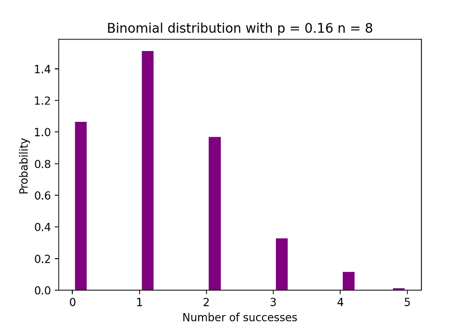
Image Source: The Author

# Random Generation of 1000 independent Binomial samples  import numpy as np  n = 8  p = 0.16  N = 1000  X = np.random.binomial(n,p,N)  # Histogram of Binomial distribution  import matplotlib.pyplot as plt  counts, bins, ignored = plt.hist(X, 20, density = True, rwidth = 0.7, color = 'purple')  plt.title("Binomial distribution with p = 0.16 n = 8")  plt.xlabel("Number of successes")  plt.ylabel("Probability")  plt.show()

Poisson Distribution

The Poisson distribution is the discrete probability distribution of the number of events occurring in a specified time period, given the average number of times the event occurs over that time period. Let's assume a random variable X follows a Poisson distribution, then the probability of observingk events over a time period can be expressed by the following probability function:

where e is Euler’s number and ? lambda, the arrival rate parameter isthe expected value of X. Poisson distribution function is very popular for its usage in modeling countable events occurring within a given time interval.

Poisson Distribution Mean & Variance

For example, Poisson distribution can be used to model the number of customers arriving in the shop between 7 and 10 pm, or the number of patients arriving in an emergency room between 11 and 12 pm. The figure below visualizes an example of Poisson distribution where we count the number of Web visitors arriving at the website where the arrival rate, lambda, is assumed to be equal to 7 minutes.

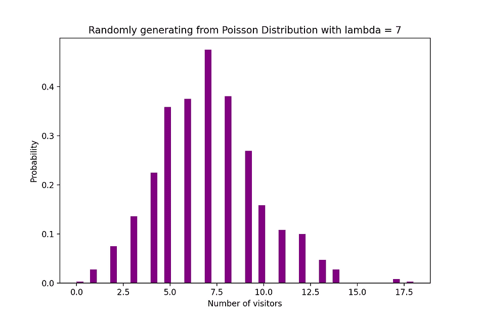
Image Source: The Author

# Random Generation of 1000 independent Poisson samples  import numpy as np  lambda_ = 7  N = 1000  X = np.random.poisson(lambda_,N)    # Histogram of Poisson distribution  import matplotlib.pyplot as plt  counts, bins, ignored = plt.hist(X, 50, density = True, color = 'purple')  plt.title("Randomly generating from Poisson Distribution with lambda = 7")  plt.xlabel("Number of visitors")  plt.ylabel("Probability")  plt.show()

Normal Distribution

The Normal probability distribution is the continuous probability distribution for a real-valued random variable. Normal distribution, also called Gaussian distribution is arguably one of the most popular distribution functions that are commonly used in social and natural sciences for modeling purposes, for example, it is used to model people’s height or test scores. Let's assume a random variable X follows a Normal distribution, then its probability density function can be expressed as follows.

where the parameter ? (mu)is the mean of the distribution also referred to as the location parameter, parameter ? (sigma)is the standard deviation of the distribution also referred to as the scale parameter. The number ? (pi) is a mathematical constant approximately equal to 3.14.

Normal Distribution Mean & Variance

The figure below visualizes an example of Normal distribution with a mean 0 (? = 0) and standard deviation of 1 (? = 1), which is referred to as Standard Normal distribution which is symmetric.

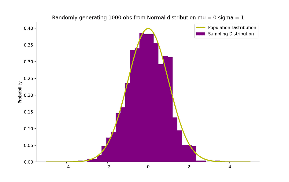
Image Source: The Author

# Random Generation of 1000 independent Normal samples  import numpy as np  mu = 0  sigma = 1  N = 1000  X = np.random.normal(mu,sigma,N)    # Population distribution  from scipy.stats import norm  x_values = np.arange(-5,5,0.01)  y_values = norm.pdf(x_values)  #Sample histogram with Population distribution  import matplotlib.pyplot as plt  counts, bins, ignored = plt.hist(X, 30, density = True,color = 'purple',label = 'Sampling Distribution')  plt.plot(x_values,y_values, color = 'y',linewidth = 2.5,label = 'Population Distribution')  plt.title("Randomly generating 1000 obs from Normal distribution mu = 0 sigma = 1")  plt.ylabel("Probability")  plt.legend()  plt.show()

Bayes Theorem

The Bayes Theorem or often called Bayes Law is arguably the most powerful rule of probability and statistics, named after famous English statistician and philosopher, Thomas Bayes.

Image Source: Wikipedia

Bayes theorem is a powerful probability law that brings the concept of subjectivity into the world of Statistics and Mathematics where everything is about facts. It describes the probability of an event, based on the prior information of conditions that might be related to that event. For instance, if the risk of getting Coronavirus or Covid-19 is known to increase with age, then Bayes Theorem allows the risk to an individual of a known age to be determined more accurately by conditioning it on the age than simply assuming that this individual is common to the population as a whole.

The concept of conditional probability, which plays a central role in Bayes theory, is a measure of the probability of an event happening, given that another event has already occurred. Bayes theorem can be described by the following expression where the X and Y stand for events X and Y, respectively:

• Pr (X|Y): the probability of event X occurring given that event or condition Y has occurred or is true
• Pr (Y|X): the probability of event Y occurring given that event or condition X has occurred or is true
• Pr (X) & Pr (Y): the probabilities of observing events X and Y, respectively

In the case of the earlier example, the probability of getting Coronavirus (event X) conditional on being at a certain age is Pr (X|Y), which is equal to the probability of being at a certain age given one got a Coronavirus, Pr (Y|X), multiplied with the probability of getting a Coronavirus, Pr (X), divided to the probability of being at a certain age., Pr (Y).

Linear Regression

Earlier, the concept of causation between variables was introduced, which happens when a variable has a direct impact on another variable. When the relationship between two variables is linear, then Linear Regression is a statistical method that can help to model the impact of a unit change in a variable, the independent variable on the values of another variable, the dependent variable.

Dependent variables are often referred to as response variables or explained variables, whereas independent variables are often referred to as regressors or explanatory variables. When the Linear Regression model is based on a single independent variable, then the model is called Simple Linear Regression and when the model is based on multiple independent variables, it’s referred to as Multiple Linear Regression. Simple Linear Regression can be described by the following expression:

where Y is the dependent variable, X is the independent variable which is part of the data, ?0 is the intercept which is unknown and constant, ?1 is the slope coefficient or a parameter corresponding to the variable X which is unknown and constant as well. Finally, u is the error term that the model makes when estimating the Y values. The main idea behind linear regression is to find the best-fitting straight line, the regression line, through a set of paired ( X, Y ) data. One example of the Linear Regression application is modeling the impact of Flipper Length on penguins’ Body Mass, which is visualized below.

Image Source: The Author

# R code for the graph  install.packages("ggplot2")  install.packages("palmerpenguins")  library(palmerpenguins)  library(ggplot2)  View(data(penguins))  ggplot(data = penguins, aes(x = flipper_length_mm,y = body_mass_g))+    geom_smooth(method = "lm", se = FALSE, color = 'purple')+    geom_point()+    labs(x="Flipper Length (mm)",y="Body Mass (g)")

Multiple Linear Regression with three independent variables can be described by the following expression:

Ordinary Least Squares

The ordinary least squares (OLS) is a method for estimating the unknown parameters such as ?0 and ?1in a linear regression model. The model is based on the principle of least squares thatminimizes the sum of squares of the differences between the observed dependent variable and its values predicted by the linear function of the independent variable, often referred to as fitted values. This difference between the real and predicted values of dependent variable Y is referred to as residual and what OLS does, is minimizing the sum of squared residuals. This optimization problem results in the following OLS estimates for the unknown parameters ?0 and ?1 which are also known as coefficient estimates.

Once these parameters of the Simple Linear Regression model are estimated, the fitted valuesof the response variable can be computed as follows:

Standard Error

The residuals or the estimated error terms can be determined as follows:

It is important to keep in mind the difference between the error terms and residuals. Error terms are never observed, while the residuals are calculated from the data. The OLS estimates the error terms for each observation but not the actual error term. So, the true error variance is still unknown. Moreover, these estimates are subject to sampling uncertainty. What this means is that we will never be able to determine the exact estimate, the true value, of these parameters from sample data in an empirical application. However, we can estimate it by calculating the sampleresidual variance by using the residuals as follows.

This estimate for the variance of sample residuals helps to estimate the variance of the estimated parameters which is often expressed as follows:

The squared root of this variance term is called the standard error of the estimate which is a key component in assessing the accuracy of the parameter estimates. It is used to calculating test statistics and confidence intervals. The standard error can be expressed as follows:

It is important to keep in mind the difference between the error terms and residuals. Error terms are never observed, while the residuals are calculated from the data.

OLS Assumptions

OLS estimation method makes the following assumption which needs to be satisfied to get reliable prediction results:

A1: Linearity assumption states that the model is linear in parameters.

A2: Random Sample assumption states that all observations in the sample are randomly selected.

A3: Exogeneity assumption states that independent variables are uncorrelated with the error terms.

A4: Homoskedasticity assumption states that the variance of all error terms is constant.

A5: No Perfect Multi-Collinearity assumption states that none of the independent variables is constant and there are no exact linear relationships between the independent variables.

def runOLS(Y,X):       # OLS esyimation Y = Xb + e --> beta_hat = (X'X)^-1(X'Y)     beta_hat = np.dot(np.linalg.inv(np.dot(np.transpose(X), X)), np.dot(np.transpose(X), Y))       # OLS prediction     Y_hat = np.dot(X,beta_hat)     residuals = Y-Y_hat     RSS = np.sum(np.square(residuals))     sigma_squared_hat = RSS/(N-2)     TSS = np.sum(np.square(Y-np.repeat(Y.mean(),len(Y))))     MSE = sigma_squared_hat     RMSE = np.sqrt(MSE)     R_squared = (TSS-RSS)/TSS       # Standard error of estimates:square root of estimate's variance     var_beta_hat = np.linalg.inv(np.dot(np.transpose(X),X))*sigma_squared_hat          SE = []     t_stats = []     p_values = []     CI_s = []          for i in range(len(beta)):         #standard errors         SE_i = np.sqrt(var_beta_hat[i,i])         SE.append(np.round(SE_i,3))            #t-statistics          t_stat = np.round(beta_hat[i,0]/SE_i,3)          t_stats.append(t_stat)            #p-value of t-stat p[|t_stat| >= t-treshhold two sided]           p_value = t.sf(np.abs(t_stat),N-2) * 2          p_values.append(np.round(p_value,3))            #Confidence intervals = beta_hat -+ margin_of_error          t_critical = t.ppf(q =1-0.05/2, df = N-2)          margin_of_error = t_critical*SE_i          CI = [np.round(beta_hat[i,0]-margin_of_error,3), np.round(beta_hat[i,0]+margin_of_error,3)]          CI_s.append(CI)          return(beta_hat, SE, t_stats, p_values,CI_s,                  MSE, RMSE, R_squared)

Parameter Properties

Under the assumption that the OLS criteria A1 — A5 are satisfied, the OLS estimators of coefficients β0 and β1 are BLUE and Consistent.

Gauss-Markov theorem

This theorem highlights the properties of OLS estimates where the term BLUE stands for Best Linear Unbiased Estimator.

Bias

The bias of an estimator is the difference between its expected value and the true value of the parameter being estimated and can be expressed as follows:

When we state that the estimator is unbiased what we mean is that the bias is equal to zero, which implies that the expected value of the estimator is equal to the true parameter value, that is:

Unbiasedness does not guarantee that the obtained estimate with any particular sample is equal or close to ?. What it means is that, if one repeatedly draws random samples from the population and then computes the estimate each time, then the average of these estimates would be equal or very close to β.

Efficiency

The term Best in the Gauss-Markov theorem relates to the variance of the estimator and is referred to as efficiency. A parameter can have multiple estimators but the one with the lowest variance is called efficient.

Consistency

The term consistency goes hand in hand with the terms sample size and convergence. If the estimator converges to the true parameter as the sample size becomes very large, then this estimator is said to be consistent, that is:

Under the assumption that the OLS criteria A1 — A5 are satisfied, the OLS estimators of coefficients β0 and β1 are BLUE and Consistent.
Gauss-Markov Theorem

All these properties hold for OLS estimates as summarized in the Gauss-Markov theorem. In other words, OLS estimates have the smallest variance, they are unbiased, linear in parameters, and are consistent. These properties can be mathematically proven by using the OLS assumptions made earlier.

Confidence Intervals

The Confidence Interval is the range that contains the true population parameter with a certain pre-specified probability, referred to as the confidence levelof the experiment, and it is obtained by using the sample results and the margin of error.

Margin of Error

The margin of error is the difference between the sample results and based on what the result would have been if one had used the entire population.

Confidence Level

The Confidence Level describes the level of certainty in the experimental results. For example, a 95% confidence level means that if one were to perform the same experiment repeatedly for 100 times, then 95 of those 100 trials would lead to similar results. Note that the confidence level is defined before the start of the experiment because it will affect how big the margin of error will be at the end of the experiment.

Confidence Interval for OLS Estimates

As it was mentioned earlier, the OLS estimates of the Simple Linear Regression, the estimates for intercept ?0 and slope coefficient ?1, are subject to sampling uncertainty. However, we can construct CI’sfor these parameters which will contain the true value of these parameters in 95% of all samples. That is, 95% confidence interval for ? can be interpreted as follows:

• The confidence interval is the set of values for which a hypothesis test cannot be rejected to the level of 5%.
• The confidence interval has a 95% chance to contain the true value of ?.

95% confidence interval of OLS estimates can be constructed as follows:

which is based on the parameter estimate, the standard error of that estimate, and the value 1.96 representing the margin of error corresponding to the 5% rejection rule. This value is determined using the Normal Distribution table, which will be discussed later on in this article. Meanwhile, the following figure illustrates the idea of 95% CI:

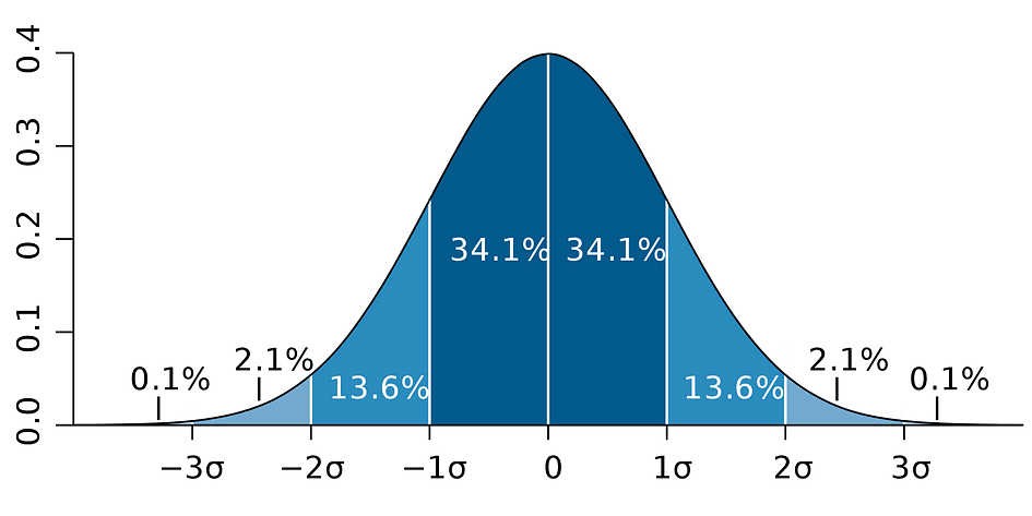
Image Source: Wikipedia

Note that the confidence interval depends on the sample size as well, given that it is calculated using the standard error which is based on sample size.

The confidence level is defined before the start of the experiment because it will affect how big the margin of error will be at the end of the experiment.

Statistical Hypothesis testing

Testing a hypothesis in Statistics is a way to test the results of an experiment or survey to determine how meaningful they the results are. Basically, one is testing whether the obtained results are valid by figuring out the odds that the results have occurred by chance. If it is the letter, then the results are not reliable and neither is the experiment. Hypothesis Testing is part of the Statistical Inference.

Null and Alternative Hypothesis

Firstly, you need to determine the thesis you wish to test, then you need to formulate the Null Hypothesis and the Alternative Hypothesis. The test can have two possible outcomes and based on the statistical results you can either reject the stated hypothesis or accept it. As a rule of thumb, statisticians tend to put the version or formulation of the hypothesis under the Null Hypothesis thatthat needs to be rejected, whereas the acceptable and desired version is stated under the Alternative Hypothesis.

Statistical significance

Let’s look at the earlier mentioned example where the Linear Regression model was used to investigating whether a penguins’ Flipper Length, the independent variable, has an impact on Body Mass, the dependent variable. We can formulate this model with the following statistical expression:

Then, once the OLS estimates of the coefficients are estimated, we can formulate the following Null and Alternative Hypothesis to test whether the Flipper Length has a statistically significant impact on the Body Mass:

where H0 and H1 represent Null Hypothesis and Alternative Hypothesis, respectively. Rejecting the Null Hypothesis would mean that a one-unit increase in Flipper Length has a direct impact on the Body Mass. Given that the parameter estimate of ?1 is describing this impact of the independent variable, Flipper Length, on the dependent variable, Body Mass. This hypothesis can be reformulated as follows:

where H0 states that the parameter estimate of ?1 is equal to 0, that is Flipper Length effect on Body Mass is statistically insignificant whereasH0 states that the parameter estimate of ?1 is not equal to 0 suggesting that Flipper Length effect on Body Mass is statistically significant.

Type I and Type II Errors

When performing Statistical Hypothesis Testing one needs to consider two conceptual types of errors: Type I error and Type II error. The Type I error occurs when the Null is wrongly rejected whereas the Type II error occurs when the Null Hypothesis is wrongly not rejected. A confusion matrix can help to clearly visualize the severity of these two types of errors.

As a rule of thumb, statisticians tend to put the version the hypothesis under the Null Hypothesis thatthat needs to be rejected, whereas the acceptable and desired version is stated under the Alternative Hypothesis.

Statistical Tests

Once the Null and the Alternative Hypotheses are stated and the test assumptions are defined, the next step is to determine which statistical test is appropriate and to calculate thetest statistic. Whether or not to reject or not reject the Null can be determined by comparing the test statistic with the critical value. This comparison shows whether or not the observed test statistic is more extreme than the defined critical value and it can have two possible results:

• The test statistic is more extreme than the critical value ? the null hypothesis can be rejected
• The test statistic is not as extreme as the critical value ? the null hypothesis cannot be rejected

The critical value is based on a prespecified significance level ? (usually chosen to be equal to 5%) and the type of probability distribution the test statistic follows. The critical value divides the area under this probability distribution curve into the rejection region(s) and non-rejection region. There are numerous statistical tests used to test various hypotheses. Examples of Statistical tests are Student’s t-test, F-test, Chi-squared test, Durbin-Hausman-Wu Endogeneity test, White Heteroskedasticity test. In this article, we will look at two of these statistical tests.

The Type I error occurs when the Null is wrongly rejected whereas the Type II error occurs when the Null Hypothesis is wrongly not rejected.

Student’s t-test

One of the simplest and most popular statistical tests is the Student’s t-test. which can be used for testing various hypotheses especially when dealing with a hypothesis where the main area of interest is to find evidence for the statistically significant effect of a single variable. Thetest statistics of the t-test follows Student’s t distribution and can be determined as follows:

where h0 in the nominator is the value against which the parameter estimate is being tested. So, the t-test statistics are equal to the parameter estimate minus the hypothesized value divided by the standard error of the coefficient estimate. In the earlier stated hypothesis, where we wanted to test whether Flipper Length has a statistically significant impact on Body Mass or not. This test can be performed using a t-test and the h0 is in that case equal to the 0 since the slope coefficient estimate is tested against value 0.

There are two versions of the t-test: a two-sided t-test and a one-sided t-test. Whether you need the former or the latter version of the test depends entirely on the hypothesis that you want to test.

The two-sidedor two-tailed t-test can be used when the hypothesis is testing equal versus not equal relationship under the Null and Alternative Hypotheses that is similar to the following example:

The two-sided t-test has two rejection regions as visualized in the figure below:

Image Source: Hartmann, K., Krois, J., Waske, B. (2018): E-Learning Project SOGA: Statistics and Geospatial Data Analysis. Department of Earth Sciences, Freie Universitaet Berlin
&nbsp

In this version of the t-test, the Null is rejected if the calculated t-statistics is either too small or too large.

Here, the test statistics are compared to the critical values based on the sample size and the chosen significance level. To determine the exact value of the cutoff point, the two-sided t-distribution table can be used.

The one-sided or one-tailed t-test can be used when the hypothesis is testing positive/negative versus negative/positive relationship under the Null and Alternative Hypotheses that is similar to the following examples:

One-sided t-test has a singlerejection region and dependingon the hypothesis side the rejection region is either on the left-hand side or the right-hand side as visualized in the figure below:

Image Source: Hartmann, K., Krois, J., Waske, B. (2018): E-Learning Project SOGA: Statistics and Geospatial Data Analysis. Department of Earth Sciences, Freie Universitaet Berlin

In this version of the t-test, the Null is rejected if the calculated t-statistics is smaller/larger than the critical value.

F-test

F-test is another very popular statistical test often used to test hypotheses testing a joint statistical significance of multiple variables. This is the case when you want to test whether multiple independent variables have a statistically significant impact on a dependent variable. Following is an example of a statistical hypothesis that can be tested using the F-test:

where the Null states that the three variables corresponding to these coefficients are jointly statistically insignificant and the Alternative states that these three variables are jointly statistically significant. The test statistics of the F-test follows F distribution and can be determined as follows:

where the SSRrestricted is the sum of squared residuals of the restricted model which is the same model excluding from the data the target variables stated as insignificant under the Null, the SSRunrestricted is the sum of squared residuals of the unrestricted modelwhich is the model that includes all variables, the q represents the number of variables that are being jointly tested for the insignificance under the Null, N is the sample size, and the k is the total number of variables in the unrestricted model. SSR values are provided next to the parameter estimates after running the OLS regression and the same holds for the F-statistics as well. Following is an example of MLR model output where the SSR and F-statistics values are marked.

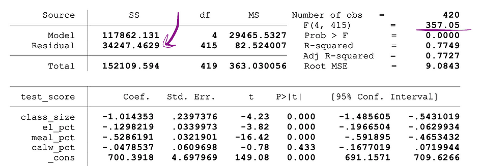
Image Source: Stock and Whatson

F-test has a single rejection region as visualized below:

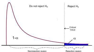
Image Source: U of Michigan

If the calculated F-statistics is bigger than the critical value, then the Null can be rejected which suggests that the independent variables are jointly statistically significant. The rejection rule can be expressed as follows:

P-Values

Another quick way to determine whether to reject or to support the Null Hypothesis is by using p-values. The p-value is the probability of the condition under the Null occurring. Stated differently, the p-value is the probability, assuming the null hypothesis is true, of observing a result at least as extreme as the test statistic. The smaller the p-value, the stronger is the evidence against the Null Hypothesis, suggesting that it can be rejected.

The interpretation of a p-value is dependent on the chosen significance level. Most often, 1%, 5%, or 10% significance levels are used to interpret the p-value. So, instead of using the t-test and the F-test, p-values of these test statistics can be used to test the same hypotheses.

The following figure shows a sample output of an OLS regression with two independent variables. In this table, the p-value of the t-test, testing the statistical significance of class_size variable’s parameter estimate, and the p-value of the F-test, testing the joint statistical significance of the class_size, and el_pct variables parameter estimates, are underlined.

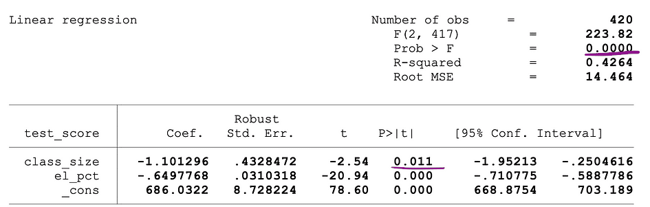
Image Source: Stock and Whatson

The p-value corresponding to the class_size variable is 0.011 and when comparing this value to the significance levels 1% or 0.01 , 5% or 0.05, 10% or 0.1, then the following conclusions can be made:

• 0.011 > 0.01 ? Null of the t-test can’t be rejected at 1% significance level
• 0.011 < 0.05 ? Null of the t-test can be rejected at 5% significance level
• 0.011 < 0.10 ?Null of the t-test can be rejected at 10% significance level

So, this p-value suggests that the coefficient of the class_size variable is statistically significant at 5% and 10% significance levels. The p-value corresponding to the F-testis 0.0000 and since 0 is smaller than all three cutoff values; 0.01, 0.05, 0.10, we can conclude that the Null of the F-test can be rejected in all three cases. This suggests that the coefficients of class_size and el_pct variables are jointly statistically significant at 1%, 5%, and 10% significance levels.

Limitation of p-values

Although, using p-values has many benefits but it has also limitations. Namely, the p-value depends on both the magnitude of association and the sample size. If the magnitude of the effect is small and statistically insignificant, the p-value might still show a significant impactbecause the large sample size is large. The opposite can occur as well, an effect can be large, but fail to meet the p<0.01, 0.05, or 0.10 criteria if the sample size is small.

Inferential Statistics

Inferential statistics uses sample data to make reasonable judgments about the population from which the sample data originated. It’s used to investigate the relationships between variables within a sample and make predictions about how these variables will relate to a larger population.

Both Law of Large Numbers (LLN) and Central Limit Theorem (CLM) have a significant role in Inferential statistics because they show that the experimental results hold regardless of what shape the original population distribution was when the data is large enough. The more data is gathered, the more accurate the statistical inferences become, hence, the more accurate parameter estimates are generated.

Law of Large Numbers (LLN)

Suppose X1, X2, . . . , Xn are all independent random variables with the same underlying distribution, also called independent identically-distributed or i.i.d, where all X’s have the same mean ? and standard deviation ?. As the sample size grows, the probability that the average of all X’s is equal to the mean ? is equal to 1. The Law of Large Numbers can be summarized as follows:

Central Limit Theorem (CLM)

Suppose X1, X2, . . . , Xn are all independent random variables with the same underlying distribution, also called independent identically-distributed or i.i.d, where all X’s have the same mean ? and standard deviation ?. As the sample size grows, the probability distribution of X converges in the distribution in Normal distribution with mean ? and variance ?-squared. The Central Limit Theorem can be summarized as follows:

Stated differently, when you have a population with mean ? and standard deviation ? and you take sufficiently large random samples from that population with replacement, then the distribution of the sample means will be approximately normally distributed.

Dimensionality Reduction Techniques

Dimensionality reduction is the transformation of data from a high-dimensional space into a low-dimensional space such that this low-dimensional representation of the data still contains the meaningful properties of the original data as much as possible.

With the increase in popularity in Big Data, the demand for these dimensionality reduction techniques, reducing the amount of unnecessary data and features, increased as well. Examples of popular dimensionality reduction techniques are Principle Component Analysis, Factor Analysis, Canonical Correlation, Random Forest.

Principle Component Analysis (PCA)

Principal Component Analysis or PCA is a dimensionality reduction technique that is very often used to reduce the dimensionality of large data sets, by transforming a large set of variables into a smaller set that still contains most of the information or the variation in the original large dataset.

Let’s assume we have a data X with p variables; X1, X2, …., Xp with eigenvectors e1, …, ep, and eigenvalues ?1,…, ?p. Eigenvalues show the variance explained by a particular data field out of the total variance. The idea behind PCA is to create new (independent) variables, called Principal Components, that are a linear combination of the existing variable. The ith principal component can be expressed as follows:

Then using Elbow Rule or Kaiser Rule, you can determine the number of principal components that optimally summarize the data without losing too much information. It is also important to look at the proportion of total variation (PRTV) that is explained by each principal component to decide whether it is beneficial to include or to exclude it. PRTV for the ith principal component can be calculated using eigenvalues as follows:

Elbow Rule

The elbow rule or the elbow method is a heuristic approach that is used to determine the number of optimal principal components from the PCA results. The idea behind this method is to plot the explained variation as a function of the number of components and pick the elbow of the curve as the number of optimal principal components. Following is an example of such a scatter plot where the PRTV (Y-axis) is plotted on the number of principal components (X-axis). The elbow corresponds to the X-axis value 2, which suggests that the number of optimal principal components is 2.

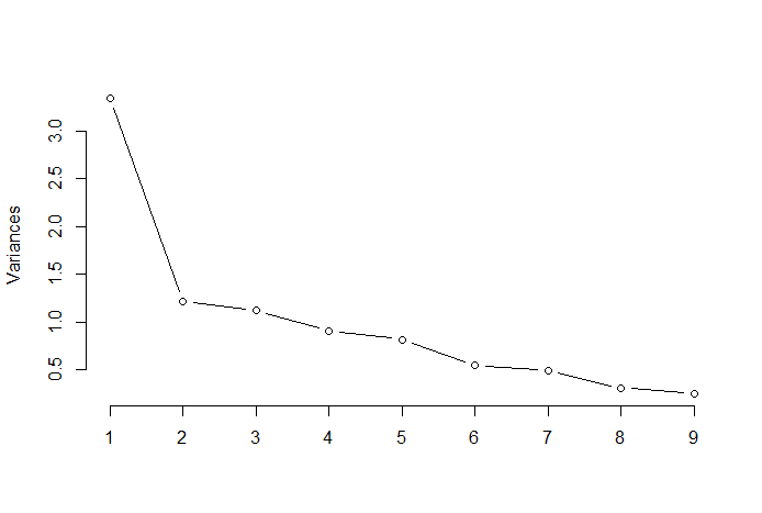
Image Source: Multivariate Statistics Github

Factor Analysis (FA)

Factor analysis or FA is another statistical method for dimensionality reduction. It is one of the most commonly used inter-dependency techniques and is used when the relevant set of variables shows a systematic inter-dependence and the objective is to find out the latent factors that create a commonality. Let’s assume we have a data X with p variables; X1, X2, …., Xp. FA model can be expressed as follows:

where X is a [p x N] matrix of p variables and N observations, µ is [p x N] population mean matrix, A is [p x k] common factor loadings matrix, F [k x N] is the matrix of common factors and u [pxN] is the matrix of specific factors. So, put it differently, a factor model is as a series of multiple regressions, predicting each of the variables Xi from the values of the unobservable common factors fi:

Each variable has k of its own common factors, and these are related to the observations via factor loading matrix for a single observation as follows: In factor analysis, the factors are calculated to maximize between-group variance while minimizing in-group variance. They are factors because they group the underlying variables. Unlike the PCA, in FA the data needs to be normalized, given that FA assumes that the dataset follows Normal Distribution.

Tatev Karen Aslanyan is an experienced full-stack data scientist with a focus on Machine Learning and AI. She is also the co-founder of LunarTech, an online tech educational platform, and the creator of The Ultimate Data Science Bootcamp.Tatev Karen, with Bachelor and Masters in Econometrics and Management Science, has grown in the field of Machine Learning and AI, focusing on Recommender Systems and NLP, supported by her scientific research and published papers. Following five years of teaching, Tatev is now channeling her passion into LunarTech, helping shape the future of data science.

Original. Reposted with permission.

More On This Topic

• Must Know for Data Scientists and Data Analysts: Causal Design Patterns
• What’s the Difference Between Data Analysts and Data Scientists?
• The Inferential Statistics Data Scientists Should Know
• Important Statistics Data Scientists Need to Know
• Practical Statistics for Data Scientists
• Will Data Analysts be Replaced by AI?

Fair Data Forecast Interview with Gregor Stühler of Scoutbee

Scoutbee’s CEO and founder, Gregor Stühler, who has a background in computer science and electrical engineering, first learned about the challenges of procurement and supply base management as a project engineer for a multinational medical device company. Scoutbee’s focus on solving supply base problems through hybrid knowledge graph and large language model (LLM) technologies reflects that understanding.

It’s not like supply chains are getting easier to manage. In this interview, Stühler states that ten years ago, companies like GE or Procter & Gamble, for example, could manage to track their top 1,000 or 2,000 suppliers with available technology. But given new regulatory requirements such as the German Supply Chain Due Diligence Act (which focuses in particular on supplier human rights compliance), the need to track multiple tiers of suppliers as well becomes necessary.

The result? Major consumer packaged goods (CPG) makers and retailers will now need to integrate and analyze millions of different data sources and data points.

Thus the growing demand for knowledge graphs (designed for ease of integration, massive scaling and ecosystem-level sharing) and contextualized data (data that is self-describing, so that one context can be easily related to others).

Scoutbee takes a practical approach to integration, one that’s based on the most important supply base management questions to answer. Each added dimension of context should provide answers to a key aspect of the supplier marketplace. The addition of a green supplier dimension, for example, suggests the need to add at least one additional data source. The data source(s) would need to answer these kinds of questions:

• How green is the supplier?
• How much money is the CPG manufacturer or retailer spending on each supplier?
• Which contracts are up for renewal?
• Which contracts should be discontinued?
• Which contracts should be initiated?

It’s interesting how Scoutbee has been acting as a mentor to customers who don’t yet have what Stühler calls “data muscle.” The company designs templates to share with customers that embody the essence of a smart, knowledge graph-enabled approach to sophisticated supply- base analytics.

Scoutbee uses AI and large language models (LLMs) to bring in and enrich the data in the knowledge graph. AI models analyze the relationships between the data points on the knowledge graph and draw conclusions. Users can query the data in the knowledge graph through Scoutbee’s new generative AI features, which gives them access to insights on their supply base in aggregate that was previously only accessible with assistance from data engineers. The combination of LLMs and knowledge graph technology helps companies unlock more contextual insights that help them drive resilience, make confident decisions, and advance their strategic priorities.

Hope you find the interview as illuminating as I have.

AI Career Notes: August 2023 Edition August 7, 2023 by Mariana Iriarte

In this monthly feature, we bring you up to date on the latest career developments in the enterprise AI community – promotions, new hires and accolades. Here's the place to read about the movers and shakers, your colleagues, your friends, and maybe yourself.

Andrew Brown

Red Hat, Inc., the provider of open source solutions, appointed Andrew Brown as its senior vice president and chief revenue officer. Brown will be responsible for commercial and public sector sales, channel and alliances sales, and consulting services, as well as the company’s global go-to-market strategy. He joins Red Hat from IBM, where he most recently served as general manager of IBM Technology Sales United Kingdom & Ireland.

“I have followed Red Hat’s growth and progress over the last few years and have been impressed by the agility, foresight, and innovative approach that the company and its culture embrace,” Brown said. “I am hugely excited about joining this unique organization and working with our customer-facing teams to innovate, collaborate and scale the hybrid cloud solutions Red Hat possesses in its open source platform approach.”

Kevin Dallas

EnterpriseDB appointed Kevin Dallas as its new chief executive officer and member of the company's board of directors. Dallas brings three decades of experience driving digital innovation and growth at technology companies, most recently as CEO at Wind River, a TPG portfolio company.

"It is an honor and a privilege to step in and lead the company's next phase focused on the intersection of data and AI," said Dallas. “The growth opportunity ahead is significant, and we continue to drive innovation to accelerate our customers’ digital transformations. I look forward to working with our talented team, the Board, Bain Capital and Great Hill Partners to realize the company’s full potential in the growing intelligent systems economy.”

Joanna Daly

Elastic, the company behind Elasticsearch, appointed Joanna Daly as its chief human resources officer. Daly has more than 20 years of global HR experience, including HR leadership roles in IBM’s consulting and technology businesses and the company’s compensation and talent organizations.

“I am honored to join Elastic, an organization recognized as a great place to work, to support the company’s next phase of growth,” said Daly. “The innovative spirit that is characteristic of the Elastic brand is what allows Elasticians to thrive and grow and help customers deliver on the promise of technologies like Generative AI—today. I am excited to build on this strong foundation of care for technology, customers, and people.”

Douglas Eadline and Jaime Hampton

Tabor Communications appointed Douglas Eadline as the Managing Editor of HPCwire. Eadline began his career as Analytical Chemist with an interest in high performance computer methods. Starting with the first Beowulf “How-To” document, he has written hundreds of articles, white papers, and instructional documents and videos covering many aspects of Linux HPC, Hadoop, and Data Analytics computing.

Tabor Communications promoted writer and editor Jaime Hampton to Managing Editor of EnterpriseAI. Hampton started with Tabor Communications as an Editorial Assistant in 2021 and was promoted to Staff Writer in 2022. This latest promotion to Managing Editor of EnterpriseAI will allow her to focus exclusively on enterprise artificial intelligence.

Casey George

Qlik appointed Casey George as its executive vice president of global sales. Casey brings over 20 years of experience scaling SaaS companies and a proven track record of earning customer loyalty and accelerating growth, most recently as chief revenue officer for Talend.

“When Qlik and Talend came together, we created a truly unique best-in-class set of data integration, data quality and analytics solutions that has the opportunity to redefine the industry,” said George. “There has never been a more exciting time to be in the data and analytics space, and I look forward to driving and expanding our leadership with our dynamic global sales organization and incredible partner ecosystem.”

Phil Guido

AMD appointed Phil Guido as its executive vice president and chief commercial officer. Guido joins AMD after more than 30 years at IBM where he most recently served as general manager, global managing partner of strategic sales at IBM Consulting.

“I am excited to welcome Phil to our leadership team as we take the next steps in our journey to make AMD the commercial and data center compute partner of choice,” said AMD chair and chief executive officer, Dr. Lisa Su. “Phil brings extensive enterprise and sales experience that will be incredibly valuable as we focus on deepening our enterprise partnerships and accelerating our growth in the data center, embedded and commercial markets. I also want to thank Darren for his transformational leadership as chief sales officer over the last eight years, and I look forward to leveraging his significant industry experience to lead strategic partnerships in his new role.”

Philippe Jeannot

2CRSi, a designer and manufacturer of high performance energy-efficient computer servers, appointed Philippe Jeannot as its deputy chief executive officer. Jeannot will manage the entire Group and its subsidiaries and be responsible for all operational, administrative, and sales activities.

"I am very pleased to be joining the 2CRSi group, and look forward to taking the opportunity to support its industrial refocusing. I hope that my experience will be of benefit to the teams," said Jeannot. “As can be seen from my career path, I am committed to improving processes, supporting company transformations and helping to improve their long-term performance.”

Simon Jesenko

Iceotope Technologies Limited, the solutions provider of precision liquid-cooling technology, appointed Simon Jesenko as its chief financial officer. Jesenko joins the company from predictive maintenance specialists Senseye, where he oversaw the company’s acquisition and integration into Siemens.

“We find ourselves at a pivotal moment in the market, where the pull towards liquid cooling solutions is accelerating as a result of two key factors: a) sustainability initiatives and regulation imposed by governments and b) an increase in computing power to accommodate processing-intensive applications, such as AI and advanced analytics,” Jesenko said. “Iceotope’s precision liquid cooling technology is at the forefront of existing liquid cooling technologies and therefore places the company in a unique position to seize this huge opportunity. My focus is going to be on delivering growth and financial performance that will increase shareholder value in the years to come as well as building a robust business structure to support this exponential growth along the way.”

Melissa Lora

Nvidia appointed Melissa Lora to its board of directors. Lora spent three decades as an executive at Taco Bell Corp., a subsidiary of Yum! Brands, Inc., before retiring in 2018 as president of Taco Bell International. She has also been appointed to the board’s audit committee.

“Melissa is a great addition to our board of directors,” said Jensen Huang, founder and CEO of Nvidia. “She brings senior management and operating experience, as well as extensive finance expertise, gained in a large corporate setting. We will benefit immensely from her guidance.”

Tim Minahan

OneStream Software, a provider of corporate performance management solutions to the world’s largest enterprises, appointed Tim Minahan as its senior vice president and chief marketing officer. Minahan joins the company from Citrix, where he held the role of EVP of business strategy and chief marketing officer.

“Having spent the last part of my career helping to transform and modernize some of the largest and most established names in software, I was eager to join a team of hard-charging innovators on a mission to create a new kind of enterprise SaaS company,” said Minahan in a blog post. “And OneStream more than fits the bill.”

Klaus Oestermann

IGEL, the managed endpoint operating system provider for secured access to any digital workspace, appointed Klaus Oestermann as its chief executive officer. Oestermann brings a track record for scaling global software businesses while building market positions and brand value. He was selected by the IGEL Board to take the top executive position after being named executive chair of the board earlier this year.

“IGEL has built one of the most respected solutions in the end user compute industry,” said Oestermann. “We stand at the forefront of digital workspace OS innovation, combining engineering excellence with strategic partnerships across top hardware device manufacturers and industry software leaders. As the future of work increasingly turns to hybrid, IGEL is poised to capture a tremendous global growth opportunity. I am eager to work with the IGEL team and its great channel partners to take the company to its full potential.”

Sumit Pal

Ontotext, the provider of enterprise knowledge graph technology and semantic database engines, appointed Sumit Pal, former Gartner VP and Analyst for Data Management and Analytics has joined the company as strategic technology director. In this role, he will be responsible for educating prospects and customers on the benefits of semantic knowledge graphs and graph databases.

“Ontotext’s technology and solutions are used across the value chain of the most knowledge-intensive enterprises in many industries, including Financial Services, Healthcare, Pharma, Manufacturing, Infrastructure, Energy and Publishing. Ontotext’s technology enables them to apply cognitive technologies for large knowledge graphs, metadata management and content analytics that is proven in various enterprise environments,“ said Pal. “I am thrilled to join this progressive company and look forward to evangelizing the value that enterprises can achieve by identifying meaning across diverse datasets and massive amounts of unstructured information.”

James Petter

Snowflake, the data cloud company, appointed James Petter as vice president of EMEA sales. Most recently, Petter spent over eight years at Pure Storage, driving increased revenues across EMEA, Latin America, and APAC. Prior to this, he spent 11 years at EMC, and a further four years at Cisco.

“As a leader, I’ve always adopted the mantra of ‘serve to lead’, and at a company as innovative and disruptive as Snowflake, this will continue to remain true,” said Petter. “Snowflake is at an exciting new chapter in its journey led by developments in generative AI, LLMs and applications, and I’m thrilled to join at this stage and extend these opportunities across EMEA, helping our customers better mobilize their data.”

Rajendra Prasad

Accenture appointed Rajendra Prasad as its chief information and asset engineering officer. Prasad will oversee all internal technology development and support for Accenture systems and Accenture assets for clients.

“Rajendra’s deep expertise in artificial intelligence, automation, and intelligent assets makes him the perfect fit to accelerate our internal transformation,” said Paul Daugherty, group chief executive – Technology and chief technology officer, Accenture. “Penelope brings significant experience delivering technology and consulting services, and we are confident her leadership will enable us to unlock new innovations and new possibilities for clients. At the same time, I want to extend my deepest gratitude to Gloria Samuels for her extraordinary contributions to Accenture over the years."

Andy Sacks, Lalit Ahuja, and Elena Schtein

GridGain, the provider of the unified real-time data platform, appointed Andy Sacks as its chief revenue officer. Sacks returned to GridGain as its CRO to lead GridGain’s global revenue strategy. He spent several years as an executive vice president of sales at Alloy Technologies, Imply Data, and early-stage GridGain.

In addition, GridGain promoted Lalit Ahuja to the role of chief product and customer officer. Over the last five years in his roles as vice president of professional services and senior vice president of customer services, Ahuja has been key to GridGain’s overall product strategy, matching the company’s ongoing innovations to the evolving needs of the market and GridGain customers.

Elena Schtein was also promoted to chief financial officer at GridGain. During Schtein’s six years at GridGain as vice president of finance, she has adeptly positioned the company for financial health and continued growth despite the global pandemic and times of economic uncertainty.

Charles Sansbury

Cloudera, the data company for trusted enterprise AI, appointed Charles Sansbury as its chief executive officer. Most recently he was CEO of ASG Technologies from 2015 until its 2021 sale to Rocket Software. Prior to that, he was COO of The Attachmate Group from 2011 until its 2014 sale to MicroFocus.

“I am grateful to the board for entrusting me with the leadership of Cloudera, and I am excited about the opportunity to take the company into its next phase of growth as the trusted enterprise AI company,” said Sansbury. “I was drawn to Cloudera for the quality of its team, its world-class customers and its position as a technology leader delivering critical enterprise AI capabilities. With over 25 million terabytes of data under management, Cloudera guides many Fortune 1000 enterprises that are focused on implementing open data lakehouses as a major step toward their expanded use of artificial intelligence and machine learning. I am confident the company will continue to execute on its product leadership position and growth initiatives.”

Raejeanne Skillern

Amazon Web Services (AWS) appointed Raejeanne Skillern as its vice president and chief marketing officer. Skillern joined AWS from Flex, where she held the role of president of communications and enterprise compute.

Before Flex, she spent over 10 years at Intel Corp. holding multiple leadership positions. Her most recent role at Intel was as vice president of the cloud service provider business unit. Skillern currently serves as a member of the board of directors at Lattice Semiconductor.

Ana White

Lumen Technologies appointed Ana White as its executive vice president and chief people officer. White joined Lumen from F5, where she held the role of EVP and CPO. Her leadership experience includes 18 years at Microsoft, where she led global HR teams. Prior to joining Microsoft, she was a compensation and benefits consultant at Willis Towers Watson.

"Lumen has a winning combination of leading-edge technologies and talented employees," said White. "I look forward to elevating the critical role of HR, helping build the company culture, and being a part of Lumen's future business success."

Kathy Willing

QuiX Quantum, a provider of quantum computing hardware based on photonics solutions, appointed Kathy Willing as its chief financial officer. Willing joins QuiX Quantum from Reynen Court, a legal tech start-up based in the US and The Netherlands where she held the position of CFO.

“I am incredibly honored to join QuiX Quantum and to work alongside such an exceptional team,” said Willing. “I cannot think of a more exciting time to join a market leader in the dynamic and rapidly changing quantum computing industry, and I am looking forward to contributing to the future growth and success at QuiX Quantum.”

To read last month's edition of Career Notes, click here.

Do you know someone that should be included in next month's list? If so, send us an email at [email protected]. We look forward to hearing from you.

Related

Life sciences have undergone a radical change as a result of AI-powered protein model prediction. In 2022, protein folding models with Google DeepMind’s AlphaFold paper being the most-cited paper of the year.

It has been two years since the London-based subsidiary of Alphabet, Google DeepMind, delivered the revolutionary answer to the decades-long ‘protein-folding problem’ in the history of AI research with AlphaFold. The open-source AlphaFold can accurately predict 3D models of protein structures from 1D amino acid sequences, which is accelerating scientific research in every field of biology and life science. Since then, the framework has been used extensively to find its real-life use cases, including the prediction of protein structures of the COVID-19 outbreak—SARS-CoV-2.

Let’s take a look at some of the interesting practical applications of AlphaFold.

Read more: The Man Behind One of The Most Important AI Advancements, AlphaFold

Advancing Malaria Vaccine Development

Biochemist and professor of molecular biology at the University of Oxford Matthew Higgins are advancing malaria vaccine development using AlphaFold. The vaccine targets multiple infection stages for comprehensive protection. They struggled to understand the critical protein Pfs48/45’s structure until AlphaFold’s integration. Combining its predictions with traditional methods clarified the protein’s workings, aiding vaccine design. Higgins acknowledges AlphaFold’s occasional inaccuracies but emphasises its collaboration with other techniques. With a clear Pfs48/45 structure, they’re entering human trials. Higgins envisions AlphaFold’s role in de novo protein design, enhancing vaccine development. This AI-tool integration shifts their project from fundamental science to clinical stages, offering potential for an effective malaria vaccine.

Delivering Gene Therapy

Scientists have made a remarkable breakthrough by tapping into the extraordinary abilities of a bacterium called Photorhabdus asymbiotica, which resides within the gut of a caterpillar, adapting it to inject proteins into human cells. This breakthrough holds potential for delivering therapeutic proteins, including those for gene editing. By modifying the syringe’s tail fibers using AlphaFold, scientists achieved successful attachment to human cells, leading to precise protein delivery. They tailored the injectors to bind with cancer cells, triggering their destruction while sparing others. Researchers harnessed AlphaFold AI to modify nanosyringes with tail fibers targeting cancer cells, precisely eliminating them while sparing others. A tagging technique allowed loading toxins and gene-editing enzyme Cas9 onto syringes, triggering cell death or gene editing when introduced to human cells. The adaptable method demonstrates potential for diverse protein loading and increased dosage. Further, AlphaFold aided modifying syringes to attach to mouse cells, successfully introducing glowing proteins into neurons. While in early stages, researchers aim to optimiSe delivery efficiency and explore DNA/RNA payloads. This study showcases AlphaFold’s role in tailoring syringes for targeted gene therapy.

Drug for Liver Cancer

A team of researchers consisting led by the University of Toronto’s Acceleration Consortium director Alán Aspuru-Guzik, Chemistry Nobel laureate Michael Levitt, and Insilico Medicine founder and CEO Alex Zhavoronkov used AlphaFold to revolutionise drug discovery for hepatocellular carcinoma (HCC), the primary liver cancer type. This pioneering research employed the New York-based biotechnology company Insilico Medicine’s automated drug designing platform Pharma.AI. Using AlphaFold-derived protein structures, they rapidly designed potent inhibitors for a new HCC treatment pathway, achieving this milestone in just 30 days and seven synthesised compounds. This hints at a new era of AI-driven therapeutics poised to reshape healthcare and address critical medical needs.

Targeting Antibiotic Resistance

Scientists Marcelo Sousa and Megan Mitchell from the University of Colorado Boulder are using AlphaFold in countering this by targeting the antibiotic resistance mechanism itself. Conventional methods struggle to understand enzyme structures responsible for resistance. AlphaFold’s rapid and accurate protein structure predictions have unlocked a decade’s worth of data in minutes. Insights into these structures could pave the way to blocking resistance, and preserving antibiotic effectiveness. Marcelo Sousa and Megan Mitchell emphasize AlphaFold’s potential in tackling antibiotic-resistant infections.

Combating Neglected Diseases

DeepMind has collaborated with the nonprofit Drugs for Neglected Diseases initiative (DNDi) to tackle deadly neglected diseases in developing countries like Chagas disease, sleeping sickness and Leishmaniasis. It has already had considerable success in finding new treatments for sleeping sickness. Most notably, it has replaced melarsoprol – a toxic compound which killed one in 20 patients – with the safe drug fexinidazole, as the new standard of care for the disease.

Read more: Protein Wars Part 2: It’s OmegaFold vs AlphaFold

The post Top 5 Use Cases of AlphaFold in Life Sciences appeared first on Analytics India Magazine.

The Great 8-bit Debate of Artificial Intelligence August 7, 2023 by Waleed Atallah

(cybermagician/Shutterstock)

A grand competition of numerical representation is shaping up as some companies promote floating point data types in deep learning, while others champion integer data types.

Artificial Intelligence Is Growing In Popularity And Cost

Artificial intelligence (AI) is proliferating into every corner of our lives. The demand for products and services powered by AI algorithms has skyrocketed alongside the popularity of large language models (LLMs) like ChatGPT, and image generation models like Stable Diffusion. With this increase in popularity, however, comes an increase in scrutiny over the computational and environmental costs of AI, and particularly the subfield of deep learning.

The primary factors influencing the costs of deep learning are the size and structure of the deep learning model, the processor it is running on, and the numerical representation of the data. State-of-the-art models have been growing in size for years now, with the compute requirements doubling every 6-10 months [1] for the last decade. Processor compute power has increased as well, but not nearly fast enough to keep up with the growing costs of the latest AI models. This has led researchers to delve deeper into numerical representation in attempts to reduce the cost of AI. Choosing the right numerical representation, or data type, has incredible implications on the power consumption, accuracy, and throughput of a given model. There is, however, no singular answer to which data type is best for AI. Data type requirements vary between the two distinct phases of deep learning: the initial training phase and the subsequent inference phase.

Finding the Sweet Spot: Bit by Bit

When it comes to increasing AI efficiency, the method of first resort is quantization of the data type. Quantization reduces the number of bits required to represent the weights of a network. Reducing the number of bits not only makes the model smaller, but reduces the total computation time, and thus reduces the power required to do the computations. This is an essential technique for those pursuing efficient AI.

AI models are typically trained using single precision 32-bit floating point (FP32) data types. It was found, however, that all 32 bits aren’t always needed to maintain accuracy. Attempts at training models using half precision 16-bit floating point (FP16) data types showed early success, and the race to find the minimum number of bits that maintains accuracy was on. Google came out with their 16-bit brain float (BF16), and models being primed for inference were often quantized to 8-bit floating point (FP8) and integer (INT8) data types. There are two primary approaches to quantizing a neural network: Post-Training Quantization (PTQ) and Quantization-Aware Training (QAT). Both methods aim to reduce the numerical precision of the model to improve computational efficiency, memory footprint, and energy consumption, but they differ in how and when the quantization is applied, and the resulting accuracy.

Post-Training Quantization (PTQ) occurs after training a model with higher-precision representations (e.g., FP32 or FP16). It converts the model's weights and activations to lower-precision formats (e.g., FP8 or INT8). Although simple to implement, PTQ can result in significant accuracy loss, particularly in low-precision formats, as the model isn't trained to handle quantization errors. Quantization-Aware Training (QAT) incorporates quantization during training, allowing the model to adapt to reduced numerical precision. Forward and backward passes simulate quantized operations, computing gradients concerning quantized weights and activations. Although QAT generally yields better model accuracy than PTQ, it requires training process modifications and can be more complex to implement.

The 8-bit Debate

The AI industry has begun coalescing around two preferred candidates for quantized data types: INT8 and FP8. Every hardware vendor seems to have taken a side. In mid 2022, a paper by Graphcore and AMD[2] floated the idea of an IEEE standard FP8 datatype. A subsequent joint paper with a similar proposal from Intel, Nvidia, and Arm[3] followed shortly. Other AI hardware vendors like Qualcomm[4, 5] and Untether AI[6] also wrote papers promoting FP8 and reviewing its merits versus INT8. But the debate is far from settled. While there is no singular answer for which data type is best for AI in general, there are superior and inferior data types when it comes to various AI processors and model architectures with specific performance and accuracy requirements.

Integer Versus Floating Point

Floating point and integer data types are two ways to represent and store numerical values in computer memory. There are a few key differences between the two formats that translate to advantages and disadvantages for various neural networks in training and inference.

The differences all stem from their representation. Floating point data types are used to represent real numbers, which include both integers and fractions. These numbers can be represented in scientific notation, with a base (mantissa) and an exponent.

On the other hand, integer data types are used to represent whole numbers (without fractions). The representations result in a very large difference in precision and dynamic range. Floating point numbers have a wider dynamic range then their integer counterparts. Integer numbers have a smaller range and can only represent whole numbers with a fixed level of precision.

Integer vs Floating Point for Training

In deep learning, the numerical representation requirements differ between the training and inference phases due to the unique computational demands and priorities of each stage. During the training phase, the primary focus is on updating the model's parameters through iterative optimization, which typically necessitates higher dynamic range to ensure the accurate propagation of gradients and the convergence of the learning process. Consequently, floating-point representations, such as FP32, FP16, and even FP8 lately, should be employed during training to maintain sufficient dynamic range. On the other hand, the inference phase is concerned with the efficient evaluation of the trained model on new input data, where the priority shifts towards minimizing computational complexity, memory footprint, and energy consumption. In this context, lower-precision numerical representations, such as 8-bit integer (INT8) become an option in addition to FP8. The ultimate decision depends on the specific model and underlying hardware.

Integer vs Floating Point for Inference

The best data type for inference will vary depending on the application and the target hardware. Real-time and mobile inference services tend to use the smaller 8-bit data types to reduce memory footprint, compute time, and energy consumption while maintaining enough accuracy.

FP8 is growing increasingly popular, as every major hardware vendor and cloud service provider has addressed its use in deep learning. There are three primary flavors of FP8, defined by the ratio of exponents to mantissa. Having more exponents increases the dynamic range of a data type, so FP8 E3M4 consisting of 1 sign bit, 3 exponent bits, and 4 mantissa bits, has the smallest dynamic range of the bunch. This FP8 representation sacrifices range for precision by having more bits reserved for mantissa, which increases the accuracy. FP8 E4M3 has an extra exponent, and thus a greater range. FP8 E5M2 has the highest dynamic range of the trio, making it the preferred target for training, which requires greater dynamic range. Having a collection of FP8 representations allows for a tradeoff between dynamic range and precision, as some inference applications would benefit from the increased accuracy offered by an extra mantissa bit.

INT8, on the other hand, effectively has 1 sign bit, 1 exponent bit, and 6 mantissa bits. This sacrifices much of its dynamic range for precision. Whether or not this translates into better accuracy compared to FP8 depends on the AI model in question. And whether or not it translates into better power efficiency will depend on the underlying hardware. Research from Untether AI research[6] shows that FP8 outperforms INT8 in terms of accuracy, and for their hardware, performance and efficiency as well. Alternatively, Qualcomm research [5] had found that the accuracy gains of FP8 are not worth the loss of efficiency compared to INT8 in their hardware. Ultimately, the decision for which data type to select when quantizing for inference will often come down to what is best supported in hardware, as well as depending on the model itself.

References

[1] Compute Trends Across Three Eras Of Machine Learning, https://arxiv.org/pdf/2202.05924.pdf
[2] 8-bit Numerical Formats for Deep Neural Networks, https://arxiv.org/abs/2206.02915
[3] FP8 Formats for Deep Learning, https://arxiv.org/abs/2209.05433
[4] FP8 Quantization: The Power of the Exponent, https://arxiv.org/pdf/2208.09225.pdf
[5] FP8 verses INT8 for Efficient Deep Learning Inference, https://arxiv.org/abs/2303.17951
[6] FP8: Efficient AI Inference Using Custom 8-bit Floating Point Data Types, https://www.untether.ai/content-request-form-fp8-whitepaper

About the Author

Waleed Atallah is a Product Manager responsible for silicon, boards, and systems at Untether AI. Currently, he is rolling out Untether AI’s second generation silicon product, the speedAI family of devices. He was previously a Product Manager at Intel, where he was responsible for high-end FPGAs with high bandwidth memory. His interests span all things compute efficiency, particularly the mapping of software to new hardware architectures. He received a B.S. degree in Electrical Engineering from UCLA.

Related

Amazon’s stake in electric vehicle maker Rivian was once worth $27 billion—that was in November, shortly after its IPO. The past years, the EV maker has been constantly struggling with production, parts, and supply chain issues, resulting in Rivian’s stock price plummeting to a 52-week low in 2022.

Started originally in 1995 as an online bookstore Amazon has expanded the business alongside its flagship search with the market throughout the years. But of course not every investment has panned out well for the company.

With Amazon owning about 17% of Rivian, the investment cost the company annual loss of $2.7 billion last year–its first unprofitable year since 2014 and a record annual loss for the company. The fiasco with Rivian has led Amazon to the list of the 13 biggest electric vehicle business failures in American history.

Earlier this year, WSJ reported, Rivians plans to call off the exclusive deal with the tech giant after it ordered fewer-than-expected delivery vans. As part of a deal made in 2019, the online retailer signed on to purchase 100,000 delivery vans from the electric vehicle company, but with Amazon reportedly only meeting the bare minimum of ordering 10,000 vehicles, the two are renegotiating the initially promising agreement.

An Investment Cemetery

While Bezos finds ways to blast himself into outer space or test-driving a 13-foot robot, he simultaneously also hunts for the next company to strengthen the Amazon arsenal. Over nearly two decades, the tech giant has made over 200 investments and 106 acquisitions. While the number is praiseworthy, the aftermath of the funnelled money has not been so.

All the way back to 1999, the ecommerce giant acquired Alexa.com for $250 million. The company providing paid subscription services with SEO and analytics tools which operated for 15 years had to be eventually shut down in 2022. While the company officially did not reveal the reason for discontinuing the service, Semrush reports suggested that there had been a constant decline in its traffic over the years.

Alexa Internet was one of the lots whose graves were dug by Amazon. In 2013, Amazon acquired LiquaVista, a liquid display firm, from Samsung, aiming to furnish Kindle e-readers’ battery-efficient screens. However, evolving screen tech quickly made LiquaVista’s “electrowetting” technology obsolete. As a result, in 2018, Amazon chose to shut down the company along with multiple in-house products.

Between 2005 and 2015, Amazon invested in, acquired and rebranded 8 emerging technology brands for undisclosed amounts which turned out to be disastrous for the company’s portfolio. All of these firms eventually were shut down within a few years of Amazon’s involvement.

In 2005, Amazon bought MobiPocket. But after a decade of no updates, Amazon permanently shut down the website and servers in 2016. In 2006, TextPayMe was rebranded to Amazon Webpay but failed to garner attention and eventually axed in 2014. New-York based Touchco was another company mysteriously shut down after the acquisition, their website and YouTube page were stripped of all content in 2010.

Similarly, in 2011 Yap, a speech recognition system acquired by Amazon was discontinued by the Amazon team and started over, leading to the development of Alexa. In 2009, Amazon acquired SnapTell, a visual product search technology but was discontinued as the company merged their technology with the Amazon experience.

For reasons varying from slow sales and the rest due to the company’s shift in focus, the company has been long known for axing its innovations. In fact, Bezos famously called the e-commerce giant “the best place in the world to fail” in his 2016 shareholder letter.

The Balancing Act

Despite the setbacks, the company continues to remain a key force in the technology sector. Even though the company has a long list of failed acquisitions and investments, a number of them have worked in favour of the tech giant.

As an example, during 2018, the retail giant introduced “Part-finder,” a mobile feature enabling users to use their device’s camera to capture an item of interest. This feature empowered Amazon to conduct a swift scan, establish a match, as well as guide users towards matching items from its catalogue. Interestingly, it was built using technology developed by Partpic, one of the companies Amazon acquired in 2016.

Even though it started as an online bookstore, the company has kept up with the market’s pace all these years. As the generative AI has swept industries globally off their feet, the company is making strides in the race. In a recent episode, the company’s current CEO Andy Jassy during last week’s Thursday’s Q2 2023 earnings call, revealed that “Every single one” of Amazon’s businesses has “multiple generative AI initiatives going right now”. While the list of ‘Killed by Amazon’ ventures continues to grow, the company’s interest evolving with the industry’s paradigm shift seems to be working in its favour as a balancing act.

The post How Amazon’s Bad Investments Led it on Thin Ice appeared first on Analytics India Magazine.