Image by Editor
After reading this article, the reader will learn the following:
- Definition of correlation
- Positive Correlation
- Negative Correlation
- Uncorrelation
- Mathematical Definition of Correlation
- Python Implementation of Correlation Coefficient
- Covariance Matrix
- Python Implementation of Covariance Matrix
Correlation
Correlation measures the degree of co-movement of two variables.
Positive Correlation
If variable Y increases when variable X increases, then X and Y are positively correlated as shown below:

Positive correlation between X and Y. Image by Author. Negative Correlation
If variable Y decreases when variable X increases, then X and Y are negatively correlated as shown below:
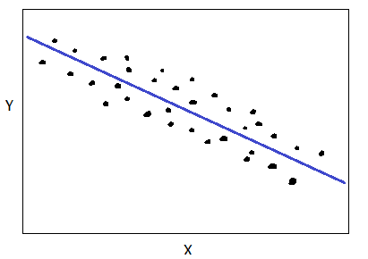
Negative correlation between X and Y. Image by Author. No correlation
When there is no obvious relationship between X and Y, we say X and Y are uncorrelated, as shown below:

X and Y are uncorrelated. Image by Author. Mathematical Definition of Correlation
Let X and Y be two features given as
X = (X1 , X2 , . . ., Xn )
Y = (Y1 , Y2 , . . ., Yn )
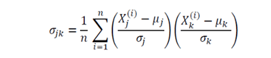
The correlation coefficient between X and Y is given as

where mu and sigma represent the mean and standard deviation, respectively, and Xstd is the standardized feature for variable X. The correlation coefficient is the vector dot product (scalar product) between the standardized features of X and Y. The correlation coefficient takes values between -1 and 1. A value close to 1 means strong positive correlation, a value close to -1 means strong negative correlation, and a value close to zero means low correlation or uncorrelation.
Python Implementation of Correlation Coefficient
import numpy as np import matplotlib.pyplot as plt n = 100 X = np.random.uniform(1,10,n) Y = np.random.uniform(1,10,n) plt.scatter(X,Y) plt.show() 
X and Y are uncorrelated. Image by Author.
X_std = (X - np.mean(X))/np.std(X) Y_std = (Y - np.mean(Y))/np.std(Y) np.dot(X_std, Y_std)/n 0.2756215872210571 # Using numpy np.corrcoef(X, Y) array([[1. , 0.27562159], [0.27562159, 1. ]])Covariance Matrix
The covariance matrix is a very useful matrix in data science and machine learning. It provides information about co-movement (correlation) between features in a dataset. The covariance matrix is given by:
where mu and sigma represent the mean and standard deviation of a given feature. Here n is the number of observations in the dataset, and the subscripts j and k take values 1, 2, 3, . . ., m, where m is the number of features in the dataset. For example, if a dataset has 4 features with 100 observations, then n = 100, and m = 4, hence the covariance matrix will be a 4 x 4 matrix. The diagonal elements will all be 1, as they represent the correlation between a feature and itself, which by definition is equal to one.
Python Implementation of the covariance matrix
Suppose I want to calculate the degree of correlation between 4 tech stocks (AAPL, TSLA, GOOGL, and AMZN) over a period of 1000 days. Our dataset has m = 4 features, and n = 1000 observations. The covariance matrix will then be a 4 x 4 matrix, as shown in the figure below.
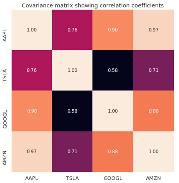
Covariance matrix between tech stocks. Image by Author.
The code for producing the figure above can be found here: Essential Linear Algebra for Data Science and Machine Learning.
Summary
In summary, we have reviewed the basics of correlation. Correlation defines the degree of co-movement between 2 variables. The correlation coefficient takes values between -1 and 1. A value close to zero means low correlation or uncorrelation.
Benjamin O. Tayo is a Physicist, Data Science Educator, and Writer, as well as the Owner of DataScienceHub. Previously, Benjamin was teaching Engineering and Physics at U. of Central Oklahoma, Grand Canyon U., and Pittsburgh State U.
- When Correlation is Better than Causation
- An Introduction to SMOTE
- An Introduction to Markov Chains
- PyCaret 101: An introduction for beginners
- A Brief Introduction to Papers With Code
- A Brief Introduction to Kalman Filters