
Image by Author Motivation
PyTorch is the most widely used Python-based Deep Learning framework. It provides tremendous support for all machine learning architectures and data pipelines. In this article, we go through all the framework basics to get you started with implementing your algorithms.
All machine learning implementations have 4 major steps:
- Data Handling
- Model Architecture
- Training Loop
- Evaluation
We go through all these steps while implementing our own MNIST image classification model in PyTorch. This will familiarize you with the general flow of a machine-learning project.
Imports
import torch import torch.nn as nn import torch.optim as optim from torch.utils.data import DataLoader # Using MNIST dataset provided by PyTorch from torchvision.datasets.mnist import MNIST import torchvision.transforms as transforms # Import Model implemented in a different file from model import Classifier import matplotlib.pyplot as plttorch.nn module provides support for neural network architectures and has built-in implementations for popular layers such as Dense Layers, Convolutional Neural Networks, and many more.
torch.optim provides implementations for optimizers such as Stochastic Gradient Descent and Adam.
Other utility modules are available for data handling support and transformations. We will go through each in more detail later.
Declare Hyperparameters
Each hyperparameter will be explained further where appropriate. However, it is a best practice to declare them at the top of our file for ease of change and understanding.
INPUT_SIZE = 784 # Flattened 28x28 images NUM_CLASSES = 10 # 0-9 hand-written digits. BATCH_SIZE = 128 # Using Mini-Batches for Training LEARNING_RATE = 0.01 # Opitimizer Step NUM_EPOCHS = 5 # Total Training EpochsData Loading and Transforms
data_transforms = transforms.Compose([ transforms.ToTensor(), transforms.Lambda(lambda x: torch.flatten(x)) ]) train_dataset = MNIST(root=".data/", train=True, download=True, transform=data_transforms) test_dataset = MNIST(root=".data/", train=False, download=True, transform=data_transforms)MNIST is a popular image classification dataset, provided by default in PyTorch. It consists of grayscale images of 10 hand-written digits from 0 to 9. Each image is of size 28 pixels by 28 pixels, and the dataset contains 60000 training and 10000 testing images.
We load the training and testing dataset separately, denoted by the train argument in the MNIST initialization function. The root argument declares the directory in which the dataset is to be downloaded.
However, we also pass an additional transform argument. For PyTorch, all inputs and outputs are supposed to be in Torch.Tensor format. This is equivalent to a numpy.ndarray in numpy. This tensor format provides additional support for data manipulation. However, the MNIST data we load from is in the PIL.Image format. We need to transform the images into PyTorch-compatible tensors. Accordingly, we pass the following transforms:
data_transforms = transforms.Compose([ transforms.ToTensor(), transforms.Lambda(lambda x: torch.flatten(x)) ])The ToTensor() transform converts images to tensor format. Next, we pass an additional Lambda transform. The Lambda function allows us to implement custom transforms. Here we declare a function to flatten the input. The images are of size 28×28, but, we flatten them i.e. convert them to a single-dimensional array of size 28×28 or 784. This will be important later when we implement our model.
The Compose function sequentially combines all the transforms. Firstly, the data is converted to tensor format and then flattened to a one-dimensional array.
Dividing our Data into Batches
For computational and training purposes, we can not pass the complete dataset into the model at once. We need to divide our dataset into mini-batches that will be fed to the model in sequential order. This allows faster training and adds randomness to our dataset, which can assist in stable training.
PyTorch provides built-in support for batching our data. The DataLoader class from torch. utils module can create batches of data, given a torch dataset module. As above, we already have the dataset loaded.
train_dataloader = DataLoader(train_dataset, batch_size=BATCH_SIZE, shuffle=True) test_dataloader = DataLoader(test_dataset, batch_size=BATCH_SIZE, shuffle=False)We pass the dataset to our dataloader, and our batch_size hyperparameter as initialization arguments. This creates an iterable data loader, so we can easily iterate over each batch using a simple for loop.
Our initial image was of size (784, ) with a single associated label. The batching then combines different images and labels in a batch. For example, if we have a batch size of 64, the input size in a batch will become (64, 784) and we will have 64 associated labels for each batch.
We also shuffle the training batch, which changes the images within a batch for each epoch. It allows for stable training and faster convergence of our model parameters.
Defining our Classification Model
We use a simple implementation consisting of 3 hidden layers. Although simple, this can give you a general understanding of combining different layers for more complex implementations.
As described above, we have an input tensor of size (784, ) and 10 different output classes, one for each digit from 0-9.
** For model implementation, we can ignore the batch dimension.
import torch import torch.nn as nn class Classifier(nn.Module): def __init__( self, input_size:int, num_classes:int ) -> None: super().__init__() self.input_layer = nn.Linear(input_size, 512) self.hidden_1 = nn.Linear(512, 256) self.hidden_2 = nn.Linear(256, 128) self.output_layer = nn.Linear(128, num_classes) self.activation = nn.ReLU() def forward(self, x): # Pass Input Sequentially through each dense layer and activation x = self.activation(self.input_layer(x)) x = self.activation(self.hidden_1(x)) x = self.activation(self.hidden_2(x)) return self.output_layer(x)Firstly, the model must inherit from the torch.nn.Module class. This provides basic functionality for neural network architectures. We then must implement two methods, __init__ and forward.
In the __init__ method, we declare all layers the model will use. We use Linear (also called Dense) layers provided by PyTorch. The first layer maps the input to 512 neurons. We can pass input_size as a model parameter, so we can later use it for input of different sizes as well. The second layer maps the 512 neurons to 256. The third hidden layer maps the 256 neurons from the previous layer to 128. The final layer then finally reduces to the output size. Our output size will be a tensor of size (10, ) because we are predicting ten different numbers.
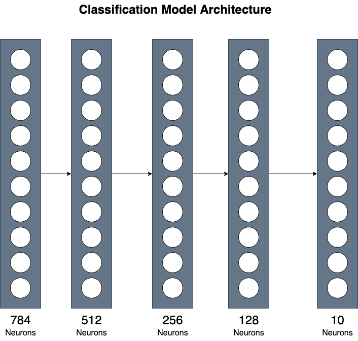
Image by Author
Moreover, we initialize a ReLU activation layer for non-linearity in our model.
The forward function receives images and we provide code for processing the input. We use the layers declared and sequentially pass our input through each layer, with an intermediate ReLU activation layer.
In our main code, we can then initialize the model providing it with the input and output size for our dataset.
model = Classifier(input_size=784, num_classes=10) model.to(DEVICE)Once initialized, we change the model device (which can be either CUDA GPU or CPU). We checked for our device when we initialized the hyperparameters. Now, we have to manually change the device for our tensors and model layers.
Training Loop
Firstly, we must declare our loss function and optimizer that will be used to optimize our model parameters.
criterion = nn.CrossEntropyLoss() optimizer = optim.Adam(model.parameters(), lr=LEARNING_RATE)Firstly, we must declare our loss function and optimizer that will be used to optimize our model parameters.
We use the Cross-Entropy Loss that is primarily used for multi-label classification models. It first applies softmax to the predictions and calculates the given target labels and predicted values.
Adam optimizer is the most-used optimizer function that allows stable gradient descent toward convergence. It is the default optimizer choice nowadays and provides satisfactory results. We pass our model parameters as an argument that denotes the weights that will be optimized.
For our training loop, we build step-by-step and fill in missing portions as we gain an understanding.
As a starting point, we iterate over the complete dataset multiple times (called epoch), and optimize our model each time. However, we have divided our data into batches. Then, for every epoch, we must iterate over each batch as well. The code for this will look as below:
for epoch in range(NUM_EPOCHS): for batch in iter(train_dataloader): # Train the Model for each batch. Now, we can train the model given a single input batch. Our batch consists of images and labels. Firstly, we must separate each of these. Our model only requires images as input to make predictions. We then compare the predictions with the true labels, to estimate our model’s performance.
for epoch in range(NUM_EPOCHS): for batch in iter(train_dataloader): images, labels = batch # Separate inputs and labels # Convert Tensor Hardware Devices to either GPU or CPU images = images.to(DEVICE) labels = labels.to(DEVICE) # Calls the model.forward() function to generate predictions predictions = model(images)We pass the batch of images directly to the model that will be processed by the forward function defined within the model. Once we have our predictions, we can optimize our model weights.
The optimization code looks as follows:
# Calculate Cross Entropy Loss loss = criterion(predictions, labels) # Clears gradient values from previous batch optimizer.zero_grad() # Computes backprop gradient based on the loss loss.backward() # Optimizes the model weights optimizer.step()Using the above code, we can compute all the backpropagation gradients and optimize the model weights using the Adam optimizer. All the above codes combined can train our model toward convergence.
Complete training loop looks as follows:
for epoch in range(NUM_EPOCHS): total_epoch_loss = 0 steps = 0 for batch in iter(train_dataloader): images, labels = batch # Separate inputs and labels # Convert Tensor Hardware Devices to either GPU or CPU images = images.to(DEVICE) labels = labels.to(DEVICE) # Calls the model.forward() function to generate predictions predictions = model(images) # Calculate Cross Entropy Loss loss = criterion(predictions, labels) # Clears gradient values from previous batch optimizer.zero_grad() # Computes backprop gradient based on the loss loss.backward() # Optimizes the model weights optimizer.step() steps += 1 total_epoch_loss += loss.item() print(f'Epoch: {epoch + 1} / {NUM_EPOCHS}: Average Loss: {total_epoch_loss / steps}')The loss gradually decreases and reaches close to 0. Then, we can evaluate the model on the test dataset we declared initially.
Evaluating our Model Performace
for batch in iter(test_dataloader): images, labels = batch images = images.to(DEVICE) labels = labels.to(DEVICE) predictions = model(images) # Taking the predicted label with highest probability predictions = torch.argmax(predictions, dim=1) correct_predictions += (predictions == labels).sum().item() total_predictions += labels.shape[0] print(f"nTEST ACCURACY: {((correct_predictions / total_predictions) * 100):.2f}")Similar to the training loop, we iterate over each batch in the test dataset for evaluation. We generate predictions for the inputs. However, for evaluation, we only need the label with the highest probability. The argmax function provides this functionality to obtain the index of the value with the highest value in our predictions array.
For the accuracy score, we can then compare if the predicted label matches the true target label. We then compute the accuracy of the number of correct labels divided by the total predicted labels.
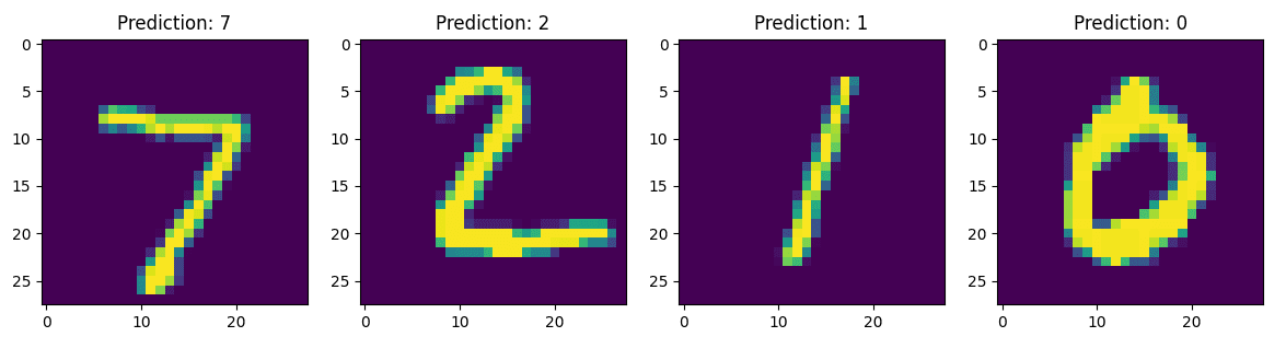
Results
I only trained the model for five epochs and achieved a test accuracy of over 96 percent, as compared to 10 percent accuracy before training. The image below shows the model predictions after training five epochs.
There you have it. You have now implemented a model from scratch that can differentiate hand-written digits just from image pixel values.
This in no way is a comprehensive guide to PyTorch but it does provide you with a general understanding of structure and data flow in a machine learning project. This is nonetheless sufficient knowledge to get you started with implementing state-of-the-art architectures in deep learning.
Complete Code
The complete code is as follows:
model.py:
import torch import torch.nn as nn class Classifier(nn.Module): def __init__( self, input_size:int, num_classes:int ) -> None: super().__init__() self.input_layer = nn.Linear(input_size, 512) self.hidden_1 = nn.Linear(512, 256) self.hidden_2 = nn.Linear(256, 128) self.output_layer = nn.Linear(128, num_classes) self.activation = nn.ReLU() def forward(self, x): # Pass Input Sequentially through each dense layer and activation x = self.activation(self.input_layer(x)) x = self.activation(self.hidden_1(x)) x = self.activation(self.hidden_2(x)) return self.output_layer(x)main.py
import torch import torch.nn as nn import torch.optim as optim from torch.utils.data import DataLoader # Using MNIST dataset provided by PyTorch from torchvision.datasets.mnist import MNIST import torchvision.transforms as transforms # Import Model implemented in a different file from model import Classifier import matplotlib.pyplot as plt if __name__ == "__main__": INPUT_SIZE = 784 # Flattened 28x28 images NUM_CLASSES = 10 # 0-9 hand-written digits. BATCH_SIZE = 128 # Using Mini-Batches for Training LEARNING_RATE = 0.01 # Opitimizer Step NUM_EPOCHS = 5 # Total Training Epochs DEVICE = 'cuda' if torch.cuda.is_available() else 'cpu' # Will be used to convert Images to PyTorch Tensors data_transforms = transforms.Compose([ transforms.ToTensor(), transforms.Lambda(lambda x: torch.flatten(x)) ]) train_dataset = MNIST(root=".data/", train=True, download=True, transform=data_transforms) test_dataset = MNIST(root=".data/", train=False, download=True, transform=data_transforms) train_dataloader = DataLoader(train_dataset, batch_size=BATCH_SIZE, shuffle=True) test_dataloader = DataLoader(test_dataset, batch_size=BATCH_SIZE, shuffle=False) model = Classifier(input_size=784, num_classes=10) model.to(DEVICE) criterion = nn.CrossEntropyLoss() optimizer = optim.Adam(model.parameters(), lr=LEARNING_RATE) for epoch in range(NUM_EPOCHS): total_epoch_loss = 0 steps = 0 for batch in iter(train_dataloader): images, labels = batch # Separate inputs and labels # Convert Tensor Hardware Devices to either GPU or CPU images = images.to(DEVICE) labels = labels.to(DEVICE) # Calls the model.forward() function to generate predictions predictions = model(images) # Calculate Cross Entropy Loss loss = criterion(predictions, labels) # Clears gradient values from previous batch optimizer.zero_grad() # Computes backprop gradient based on the loss loss.backward() # Optimizes the model weights optimizer.step() steps += 1 total_epoch_loss += loss.item() print(f'Epoch: {epoch + 1} / {NUM_EPOCHS}: Average Loss: {total_epoch_loss / steps}') # Save Trained Model torch.save(model.state_dict(), 'trained_model.pth') model.eval() correct_predictions = 0 total_predictions = 0 for batch in iter(test_dataloader): images, labels = batch images = images.to(DEVICE) labels = labels.to(DEVICE) predictions = model(images) # Taking the predicted label with highest probability predictions = torch.argmax(predictions, dim=1) correct_predictions += (predictions == labels).sum().item() total_predictions += labels.shape[0] print(f"nTEST ACCURACY: {((correct_predictions / total_predictions) * 100):.2f}") # -- Code For Plotting Results -- # batch = next(iter(test_dataloader)) images, labels = batch fig, ax = plt.subplots(nrows=1, ncols=4, figsize=(16,8)) for i in range(4): image = images[i] prediction = torch.softmax(model(image), dim=0) prediction = torch.argmax(prediction, dim=0) # print(type(prediction), type(prediction.item())) ax[i].imshow(image.view(28,28)) ax[i].set_title(f'Prediction: {prediction.item()}') plt.show()Muhammad Arham is a Deep Learning Engineer working in Computer Vision and Natural Language Processing. He has worked on the deployment and optimizations of several generative AI applications that reached the global top charts at Vyro.AI. He is interested in building and optimizing machine learning models for intelligent systems and believes in continual improvement.
- A Bug That Can Make You a Data Science Hero
- Zero to RAPIDS in Minutes with NVIDIA GPUs + Saturn Cloud
- Breaking the Data Barrier: How Zero-Shot, One-Shot, and Few-Shot Learning…
- Zero-shot Learning, Explained
- 4 Machine Learning Concepts I Wish I Knew When I Built My First Model
- How to Create Stunning Web Apps for your Data Science Projects